Quickstart
Basic usage — load data & compute derivatives
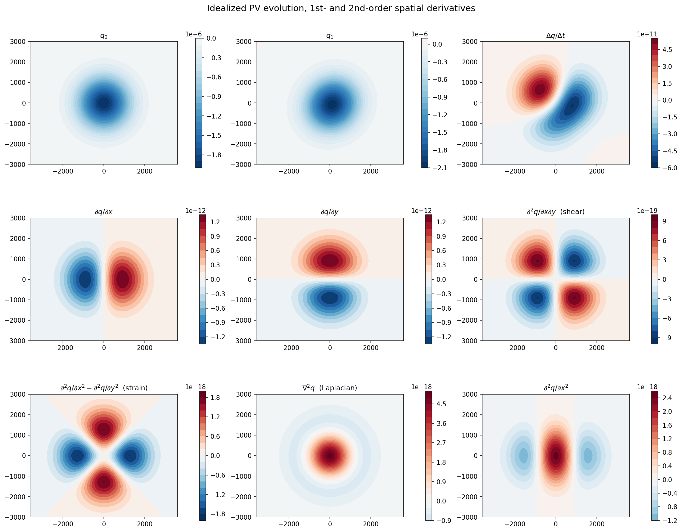
pvtend ships with an idealized Gaussian PV anomaly that undergoes
simultaneous propagation, intensification, and deformation over one
hour. Let’s load it, compute all the spatial/temporal derivatives
(including the second-order terms needed for the six-basis
decomposition), and visualise them.
import numpy as np
import matplotlib.pyplot as plt
import pvtend

# ── 1. Load bundled sample data ──────────────────────────────────
d = pvtend.load_idealized_pv()
q0, q1 = d["q0"], d["q1"]          # PV at t=0 and t=1   [PVU]
x_km, y_km = d["x_km"], d["y_km"]  # coordinate vectors   [km]
x_deg, y_deg = d["x_deg"], d["y_deg"]
dx_arr, dy_m, dt = d["dx_arr"], float(d["dy_m"]), float(d["dt"])

print(f"Grid shape: {q0.shape},  Δx = {float(d['dx_m'])/1e3:.0f} km,  Δt = {dt:.0f} s")

# ── 2. First-order derivatives ───────────────────────────────────
dq_dx = pvtend.ddx(q0, dx_arr, periodic=False)  # ∂q/∂x  [PVU/m]
dq_dy = pvtend.ddy(q0, dy_m)                     # ∂q/∂y  [PVU/m]
dq_dt = (q1 - q0) / dt                           # Δq/Δt  [PVU/s]

# ── 3. Second-order derivatives (for the six-basis fields) ───────
dq_dxdy = pvtend.ddy(dq_dx, dy_m)                              # ∂²q/∂x∂y  (Φ₄ shear)
dq_dx2  = pvtend.ddx(dq_dx, dx_arr, periodic=False)            # ∂²q/∂x²
dq_dy2  = pvtend.ddy(dq_dy, dy_m)                              # ∂²q/∂y²
strain  = dq_dx2 - dq_dy2                                      # ∂²q/∂x²−∂²q/∂y² (Φ₅ normal strain)
laplacian = dq_dx2 + dq_dy2                                    # ∂²q/∂x²+∂²q/∂y² (Φ₆ Laplacian)

# ── 4. Visualise (3 rows × 3 columns) ────────────────────────────
panels = [
    (q0,        r"$q_0$"),
    (q1,        r"$q_1$"),
    (dq_dt,     r"$\Delta q / \Delta t$"),
    (dq_dx,     r"$\partial q / \partial x$"),
    (dq_dy,     r"$\partial q / \partial y$"),
    (dq_dxdy,   r"$\partial^2 q / \partial x \partial y$  (shear)"),
    (strain,    r"$\partial^2 q/\partial x^2 - \partial^2 q/\partial y^2$  (strain)"),
    (laplacian, r"$\nabla^2 q$  (Laplacian)"),
    (dq_dx2,    r"$\partial^2 q / \partial x^2$"),
]

fig, axes = plt.subplots(3, 3, figsize=(15, 12), constrained_layout=True)
for ax, (fld, title) in zip(axes.ravel(), panels):
    vm = np.nanmax(np.abs(fld)) or 1.0
    im = ax.contourf(x_km, y_km, fld, 21, vmin=-vm, vmax=vm, cmap="RdBu_r")
    ax.set_title(title, fontsize=11)
    ax.set_aspect("equal")
    plt.colorbar(im, ax=ax, shrink=0.75)
fig.suptitle("Idealized PV evolution, 1st- and 2nd-order spatial derivatives", fontsize=14)
plt.show()
Orthogonal basis decomposition
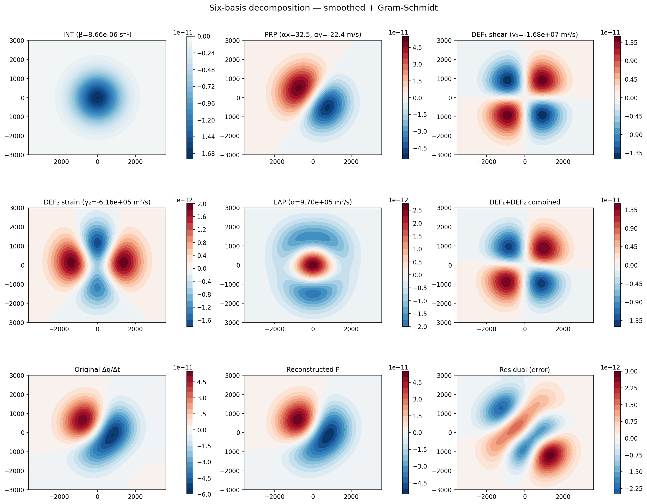
Using the derivatives from above, build the six orthogonal bases (Φ₁ intensification / Φ₂–Φ₃ propagation / Φ₄–Φ₅ deformation / Φ₆ Laplacian) via Gram-Schmidt, project the PV tendency, and compare the reconstruction with the original.
from pvtend import compute_orthogonal_basis, project_field

# ── 1. Build orthogonal basis ────────────────────────────────────
#   pv_anom = q0  (the anomaly at t=0)
#   smoothing_deg and grid_spacing are in degrees
grid_sp = float(d["grid_spacing_deg"])

basis = compute_orthogonal_basis(
    pv_anom=q0,
    pv_dx=dq_dx,
    pv_dy=dq_dy,
    x_rel=x_deg,
    y_rel=y_deg,
    mask="< 0",
    apply_smoothing=True,
    smoothing_deg=3.0,
    grid_spacing=grid_sp,
)

# ── 2. Project tendency onto basis ───────────────────────────────
result = project_field(dq_dt, basis)

print(f"β  (intensification)     = {result['beta']:.3e} s⁻¹")
print(f"αx (zonal propagation)   = {result['ax']:.1f} m/s")
print(f"αy (merid. propagation)  = {result['ay']:.1f} m/s")
print(f"γ₁ (shear deformation)   = {result['gamma1']:.3e} m² s⁻¹")
print(f"γ₂ (normal strain)       = {result['gamma2']:.3e} m² s⁻¹")
print(f"σ  (Laplacian/diffusion) = {result['sigma']:.3e} m² s⁻¹")
print(f"RMSE                     = {result['rmse']:.3e}")

# ── 3. Visualise (3 rows × 3 columns) ────────────────────────────
panels2 = [
    (result["int"],   rf"INT ($\beta$={result['beta']:.2e} s$^{{-1}}$)"),
    (result["prop"],  rf"PRP ($\alpha_x$={result['ax']:.1f}, $\alpha_y$={result['ay']:.1f} m/s)"),
    (result["def1"],  rf"DEF$_1$ shear ($\gamma_1$={result['gamma1']:.2e} m$^2$/s)"),
    (result["def2"],  rf"DEF$_2$ strain ($\gamma_2$={result['gamma2']:.2e} m$^2$/s)"),
    (result["lap"],   rf"LAP ($\sigma$={result['sigma']:.2e} m$^2$/s)"),
    (result["def"],   r"DEF$_1$+DEF$_2$ combined"),
    (dq_dt,           r"Original $\Delta q / \Delta t$"),
    (result["recon"], r"Reconstructed $\hat{F}$"),
    (result["resid"], "Residual (error)"),
]

fig, axes = plt.subplots(3, 3, figsize=(15, 12), constrained_layout=True)
for ax, (fld, title) in zip(axes.ravel(), panels2):
    vm = np.nanmax(np.abs(fld)) or 1.0
    im = ax.contourf(x_km, y_km, fld, 21, vmin=-vm, vmax=vm, cmap="RdBu_r")
    ax.set_title(title, fontsize=11)
    ax.set_aspect("equal")
    plt.colorbar(im, ax=ax, shrink=0.75)
fig.suptitle("Six-basis decomposition — smoothed + Gram-Schmidt", fontsize=14)
plt.show()
Command-line pipeline
The full production pipeline is a three-pass workflow:
Pre-compute Helmholtz climatology (one-time) — decompose the climatological (ū, v̄) into rotational / divergent parts for each month. Results are cached as 24 NetCDF files (~seconds).
Compute (Pass 0) — extract PV tendency terms for each tracked event into per-timestep NPZ files. This is the most expensive step; with
--n-workers 48it takes ~12 hours for ~500 events.Classify (Pass 1) — detect Rossby Wave Breaking on the NPZ patches and label each event as AWB, CWB, or neutral (~minutes).
Composite (Pass 2) — accumulate NPZ fields into variant-aware composites, stratified by RWB type (~seconds).
# ── Pass 0a: Pre-compute Helmholtz climatology (one-time) ────────
pvtend-pipeline clim-helmholtz \
    --clim-dir /path/to/climatology/ \
    --output-dir /path/to/climatology/ \
    --clim-stem era5_hourly_clim_1990-2020

# ── Pass 0: Compute PV tendencies ────────────────────────────────
# Recommended: 48 parallel workers → ~12 h for ~500 blocking events
pvtend-pipeline compute \
    --event-type blocking \
    --events-csv tracked_events.csv \
    --era5-dir /path/to/era5/ \
    --clim-path /path/to/climatology/era5_hourly_clim.nc \
    --clim-helmholtz-dir /path/to/climatology/ \
    --out-dir /path/to/output/ \
    --dh-range='-49:25:1' \
    --center-mode eulerian \
    --year-range '1990:2011' \
    --stages onset peak decay \
    --n-workers 48 \
    --skip-existing

# ── Pass 1: RWB classification ───────────────────────────────────
#   Detects overturning Z contours on multiple pressure levels and
#   classifies each event-stage as AWB / CWB / Omega (both) / NEUTRAL.
#   --levels accepts integer hPa values or 'wavg' (weighted-average Z).
pvtend-pipeline classify \
    --npz-dir /path/to/output/ \
    --output /path/to/outputs/rwb_variant_tracksets.pkl \
    --levels 500 400 300 200 \
    --threshold 3

# Single-field "wavg one level" mode (e.g. for the upper-trop 300/250/200
# weighted-average Z): one field, threshold clamps to 1.
pvtend-pipeline classify --npz-dir /path/to/output/ \
    --output /path/to/outputs/rwb_wavg.pkl --levels wavg --threshold 1

# Second option — classify a pre-extracted patch file (.npz or .nc) of
# single 2-D Z fields built on ANY grid (e.g. CESM f09), writing a per-event
# AWB/CWB/Omega/NEUTRAL label CSV (npz tree stays the default):
pvtend-pipeline classify \
    --patches /path/to/zwavg_patches.npz \
    --output /path/to/outputs/rwb_labels.csv
# In Python, the same single-field classifier is the public
#   pvtend.classify.classify_z_field(z2d, x_rel, y_rel) -> (awb, cwb)
#   pvtend.classify.label_from_flags(awb, cwb) -> "AWB"/"CWB"/"Omega"/"NEUTRAL"

# ── Pass 2: Variant-aware composite ──────────────────────────────
#   Accumulates NPZ fields, separately for "original", "AWB_onset",
#   "CWB_peak", etc.  Produces a single composite.pkl.
pvtend-pipeline composite \
    --npz-dir /path/to/output/ \
    --rwb-pkl /path/to/outputs/rwb_variant_tracksets.pkl \
    --pkl-out /path/to/outputs/composite_blocking.pkl

# ── (Optional) Pass 3: Orthogonal basis decomposition ────────────
pvtend-pipeline decompose \
    --pkl-in /path/to/outputs/composite_blocking.pkl \
    --out-dir /path/to/outputs/decomposition/
The resulting composite_blocking.pkl can be loaded and inspected in
Python:
from pvtend import load_composite_state

comp = load_composite_state("composite_blocking.pkl")

# Get composite-mean PV at peak + 0 h for AWB events
pv_awb = comp.composite_mean_3d("pv_3d", stage="peak", dh=0, variant="AWB_peak")
Per-level piecewise PV inversion (PPVI)
The pvtend.ppvi subpackage adds piecewise potential-vorticity
inversion (Wu/Davis nonlinear balance) to each event NPZ: it decomposes the
balanced rotational-wind anomaly into the contribution induced by each
pressure level’s PV / boundary-θ anomaly, across the 9 Wu levels
1000 → 100 hPa. The 1000 hPa (bottom-θ) and 100 hPa (top-θ) pieces are
Bretherton (1966) boundary sheets; levels 2–8 are interior PV. Because the
perturbation balance is linear, the 9 single-level pieces sum exactly to the
full balanced field.
Per-event NPZ keys (for L in {1000, 850, 700, 500, 400, 300, 250, 200,
100}):
u_rot_anom_ppvi_{L}/v_rot_anom_ppvi_{L}(+_3d) — rotational-wind anomaly induced by inverting only levelL’s PV/θ piece;u/v_rot_anom_residual_ppvi— observed minus the sum of all per-level pieces (the unbalanced / divergent part);pv_anom_wu— the Wu PV anomaly that is inverted.
PPVI runs by default in compute (disable with --no-with-ppvi); to
add it to existing NPZ (or recompute), use the ppvi subcommand. The Wu
inversion can occasionally segfault on a few events; the fault-tolerant pool
retries and --skip-existing makes the run idempotent/resumable. Because a
long-lived worker accumulates per-event reads, run very large migrations in
chunks (a few hundred events per invocation):
# add / replace per-level PPVI fields in existing event NPZ (resumable)
pvtend-pipeline ppvi \
    --event-type blocking \
    --events-csv tracked_events.csv \
    --era5-dir /path/to/era5/ \
    --clim-path /path/to/climatology/era5_hourly_clim_1990-2020 \
    --clim-helmholtz-dir /path/to/climatology/ \
    --out-dir /path/to/output/ \
    --dh-range='-12:13' \
    --n-workers 192 \
    --skip-existing
The per-level decomposition shows, e.g., that a blocking ridge’s 250 hPa circulation is driven mostly by the 250/200/300 hPa PV pieces, while the warm-core 1000 hPa piece is weak and of opposite sign aloft.