02 — Helmholtz Decomposition, QG Omega & PV Tendency
End-to-end demonstration on ERA5 January 2025 data (Northern Hemisphere, 1.5°, 9 levels).
Pipeline (matches core/step2_compute_tendency_terms_blocking.py):
Load raw ERA5 fields on full NH grid (61×240)
Helmholtz decomposition on total wind (u, v) on full NH (spherical FFT Laplacian, requires full longitude ring)
PV spatial derivatives (∂q/∂x, ∂q/∂y, ∂q/∂p) on full NH (periodic zonal boundaries)
Extract event-centred patch (±21° lat × ±36° lon → 29×49) at California / East Pacific
QG omega on full NH: SP19 (scaling) and LOG20 (SIP) for ω_adia (A+B terms)
Three omega components: ω_adia, ω_qg_diabatic, ω_lhr_moist (LHR via C term)
Diabatic / adiabatic divergent wind via independent Poisson inversions using ω_lhr_moist on patch
PV tendency: LHR-moist indirect contribution vs total divergent outflow on patch (total PV gradients)
Save NPZ of all computed fields
[1]:
import numpy as np
import xarray as xr
import matplotlib.pyplot as plt
import cartopy.io.shapereader as shpreader
from shapely.geometry import box as shapely_box
import time, gc

from pvtend import (
    NHGrid, EventPatch,
    R_EARTH, OMEGA_E, R_DRY, KAPPA, G0, SP19_DRY_FRACTION,
    helmholtz_decomposition_3d, solve_qg_omega_sip, decompose_omega,
    ddx, ddy, ddp,
)
from pvtend.helmholtz import gradient, solve_poisson_spherical_fft, laplacian_spherical_fft
from pvtend.derivatives import gradient_periodic
from pvtend.moist_dry import solve_chi_from_omega
from pvtend.omega import _compute_diabatic_rhs_emanuel


# ── Coastline overlay in event-relative coordinates ──
def overlay_coastlines(ax, centre_lat, centre_lon, xlim, ylim,
                       lw=0.5, color="k", alpha=0.6, resolution="50m"):
    """Overlay coastlines in event-relative coordinates."""
    shp = shpreader.natural_earth(resolution, "physical", "coastline")
    reader = shpreader.Reader(shp)
    clip = shapely_box(centre_lon + xlim[0], centre_lat + ylim[0],
                       centre_lon + xlim[1], centre_lat + ylim[1])
    for geom in reader.geometries():
        clipped = geom.intersection(clip)
        if clipped.is_empty:
            continue
        parts = clipped.geoms if hasattr(clipped, "geoms") else [clipped]
        for part in parts:
            if hasattr(part, "coords"):
                coords = np.array(part.coords)
                ax.plot(coords[:, 0] - centre_lon,
                        coords[:, 1] - centre_lat,
                        color=color, lw=lw, alpha=alpha)


%matplotlib inline
plt.rcParams.update({"figure.dpi": 120, "font.size": 10})
1 Load ERA5 January 2025 & set up grid
All data on full NH grid (61 lat × 240 lon, 1.5°). NHGrid and EventPatch are configured for later patch extraction.
[2]:
# ══════════════════════════════════════════════════════════════
# Configuration (change freely)
# ══════════════════════════════════════════════════════════════
DATA_DIR    = "era5_jan2025"
TIME_IDX    = 252               # snapshot index (≈ 2025-01-15 12Z)
PLOT_LEV    = 300               # hPa for all map plots
CENTER_LAT  = 40.0              # event centre latitude [°N]
CENTER_LON  = -120.0            # event centre longitude [°E]
QG_METHOD   = "log20"            # "sp19" (scaling) or "log20" (SIP solver)

# ══════════════════════════════════════════════════════════════
# Load all variables (full NH)
# ══════════════════════════════════════════════════════════════
print("Loading ERA5 data …")
ds_u  = xr.open_dataset(f"{DATA_DIR}/era5_u_2025_01.nc")
ds_v  = xr.open_dataset(f"{DATA_DIR}/era5_v_2025_01.nc")
ds_t  = xr.open_dataset(f"{DATA_DIR}/era5_t_2025_01.nc")
ds_z  = xr.open_dataset(f"{DATA_DIR}/era5_z_2025_01.nc")
ds_w  = xr.open_dataset(f"{DATA_DIR}/era5_w_2025_01.nc")
ds_pv = xr.open_dataset(f"{DATA_DIR}/era5_pv_2025_01.nc")

# Coordinates: flip latitude to ascending, pressure to Pa
lat_raw  = ds_u["latitude"].values          # 90 → 0 (descending)
lon      = ds_u["longitude"].values         # -180 → 178.5
levs_hpa = ds_u["pressure_level"].values    # [1000, 850, …, 100]
times    = ds_u["valid_time"].values

flip     = lat_raw[0] > lat_raw[-1]
lat      = lat_raw[::-1] if flip else lat_raw       # ascending 0 → 90
plevs_pa = (levs_hpa * 100.0).astype(np.float64)    # Pa, ascending
nlev, nlat, nlon = len(levs_hpa), len(lat), len(lon)

def _load(ds, var):
    """Load 4-D array → (nt, nlev, nlat, nlon) with ascending lat."""
    arr = ds[var].values.astype(np.float32)
    return arr[:, :, ::-1] if flip else arr

u_all  = _load(ds_u,  "u")
v_all  = _load(ds_v,  "v")
t_all  = _load(ds_t,  "t")
z_all  = _load(ds_z,  "z")        # geopotential Φ [m²/s²]
w_all  = _load(ds_w,  "w")        # omega ω [Pa/s]
pv_all = _load(ds_pv, "pv")       # potential vorticity [PVU]

for ds in [ds_u, ds_v, ds_t, ds_z, ds_w, ds_pv]:
    ds.close()

# ── Snapshot ──
ts_str  = str(times[TIME_IDX])[:16]
u_snap, v_snap = u_all[TIME_IDX], v_all[TIME_IDX]
t_snap, z_snap = t_all[TIME_IDX], z_all[TIME_IDX]
w_snap, pv_snap = w_all[TIME_IDX], pv_all[TIME_IDX]

del u_all, v_all, t_all, z_all, w_all, pv_all
gc.collect()

# ══════════════════════════════════════════════════════════════
# NH grid & EventPatch setup
# ══════════════════════════════════════════════════════════════
grid    = NHGrid(lat=lat, lon=lon)          # NHGrid works with ascending too
patcher = EventPatch(grid)                  # ±21° lat × ±36° lon

ilev = np.argmin(np.abs(levs_hpa - PLOT_LEV))

# ── Grid spacing (full NH, ascending lat) ──
lat_rad = np.deg2rad(lat)
dlat = float(np.abs(lat[1] - lat[0]))
dlon = float(np.abs(lon[1] - lon[0]))
dy     = np.deg2rad(dlat) * R_EARTH
dx_arr = np.deg2rad(dlon) * R_EARTH * np.cos(lat_rad)
dx_arr = np.maximum(dx_arr, dy * 0.1)

# ── Coriolis (full NH) ──
f_arr   = 2.0 * OMEGA_E * np.sin(lat_rad)
f_clamp = 2.0 * OMEGA_E * np.sin(np.deg2rad(5.0))
f_arr   = np.where(np.abs(f_arr) < f_clamp,
                   np.sign(f_arr + 1e-30) * f_clamp, f_arr)

print(f"Full NH grid: {nlat}×{nlon}, {nlev} levels ({levs_hpa} hPa)")
print(f"Snapshot: {ts_str}  |  PLOT_LEV = {PLOT_LEV} hPa")
print(f"Event centre: ({CENTER_LAT}°N, {CENTER_LON}°E)")
print(f"Patch shape: {patcher.patch_shape}")
print(f"|u_snap| max = {np.abs(u_snap).max():.1f} m/s  |  |w_snap| max = {np.abs(w_snap).max():.4f} Pa/s")
Loading ERA5 data …
Full NH grid: 61×240, 9 levels ([1000.  850.  700.  500.  400.  300.  250.  200.  100.] hPa)
Snapshot: 2025-01-15T12:00  |  PLOT_LEV = 300 hPa
Event centre: (40.0°N, -120.0°E)
Patch shape: (29, 49)
|u_snap| max = 101.2 m/s  |  |w_snap| max = 6.3439 Pa/s
2 Helmholtz decomposition on full NH grid
Splits total wind (u, v) at each level into rotational (ψ), divergent (χ), and harmonic components. Since v2.10 helmholtz_decomposition_3d defaults to method="spectral" (spherical-harmonic backend via pvtend.sh_ops, pyspharm) which parity-mirrors the NH input to the global sphere; the legacy spherical-FFT Poisson path (conservative form, following xinvert/MiniUFO) is still available as method="fft". Either path needs the full NH grid (full longitude ring) for
the periodic zonal BCs.
[3]:
%%time
# Full NH Helmholtz on TOTAL wind (default: SH spectral backend via pyspharm; method="fft" for legacy spherical-FFT): (nlev, 61, 240) → dict of same shape
helm = helmholtz_decomposition_3d(u_snap, v_snap, lat, lon)
print("Helmholtz output keys:", sorted(helm.keys()))

print(f"\nAt {PLOT_LEV} hPa (level index {ilev}):")
for comp in ["u_rot", "v_rot", "u_div", "v_div", "u_har", "v_har"]:
    print(f"  {comp:6s}  range = [{helm[comp][ilev].min():.3f}, {helm[comp][ilev].max():.3f}] m/s")
print(f"  psi    range = [{helm['psi'][ilev].min():.3e}, {helm['psi'][ilev].max():.3e}] m²/s")
print(f"  chi    range = [{helm['chi'][ilev].min():.3e}, {helm['chi'][ilev].max():.3e}] m²/s")
Helmholtz output keys: ['chi', 'divergence', 'psi', 'u_div', 'u_har', 'u_rot', 'v_div', 'v_har', 'v_rot', 'vorticity']

At 300 hPa (level index 5):
  u_rot   range = [-40.222, 97.541] m/s
  v_rot   range = [-58.882, 63.819] m/s
  u_div   range = [-15.449, 16.047] m/s
  v_div   range = [-17.042, 16.704] m/s
  u_har   range = [-3.388, 2.939] m/s
  v_har   range = [-4.219, 4.375] m/s
  psi    range = [-1.539e+08, 2.585e+07] m²/s
  chi    range = [-1.617e+07, 2.439e+07] m²/s
CPU times: user 55.7 ms, sys: 4.27 ms, total: 60 ms
Wall time: 60.7 ms
3 PV spatial derivatives on full NH grid
Compute \(\partial q/\partial x\), \(\partial q/\partial y\), \(\partial q/\partial p\) on the full NH domain using periodic zonal boundaries. Uses the total PV field (pv_snap).
[4]:
# ── PV gradients on full NH (periodic lon) ──
# Total PV derivatives (bar = total field treated as background)
dpv_bar_dx = np.zeros_like(pv_snap)
dpv_bar_dy = np.zeros_like(pv_snap)
for k in range(nlev):
    dpv_bar_dx[k], dpv_bar_dy[k] = gradient_periodic(pv_snap[k], dx_arr, dy)

# ∂q_bar/∂p  (centred finite differences)
dpv_bar_dp = np.zeros_like(pv_snap)
for k in range(1, nlev - 1):
    dpv_bar_dp[k] = (pv_snap[k+1] - pv_snap[k-1]) / (plevs_pa[k+1] - plevs_pa[k-1])
dp_fd = np.diff(plevs_pa)
dpv_bar_dp[0]  = (pv_snap[1]  - pv_snap[0])  / dp_fd[0]
dpv_bar_dp[-1] = (pv_snap[-1] - pv_snap[-2]) / dp_fd[-1]

print("Full-NH PV derivatives computed:")
print(f"  |∂q/∂x| max = {np.abs(dpv_bar_dx[ilev]).max():.4e}")
print(f"  |∂q/∂y| max = {np.abs(dpv_bar_dy[ilev]).max():.4e}")
print(f"  |∂q/∂p| max = {np.abs(dpv_bar_dp[ilev]).max():.4e}")
Full-NH PV derivatives computed:
  |∂q/∂x| max = 4.0278e-11
  |∂q/∂y| max = 2.5321e-11
  |∂q/∂p| max = 5.8584e-10
4 Extract event-centred patch
Centre the ±21° lat × ±36° lon patch on California / East Pacific. Crop all full-NH fields (Helmholtz winds, PV derivatives, meteorological vars) to this patch. Compute geostrophic wind on the patch (matching core/step2 pipeline).
[5]:
# ── Find patch centre index ──
i_lat, i_lon, ok = patcher.nearest_idx(CENTER_LAT, CENTER_LON)
assert ok, f"Patch does not fit at ({CENTER_LAT}, {CENTER_LON})"

# ── Relative grid ──
Y_rel, X_rel = patcher.relative_grid()
x_coords = X_rel[0, :]    # 1D relative longitude
y_coords = Y_rel[:, 0]    # 1D relative latitude

# ── Coastline overlay kwargs (reused in all plots) ──
coast_kw = dict(centre_lat=CENTER_LAT, centre_lon=CENTER_LON,
                xlim=(x_coords.min(), x_coords.max()),
                ylim=(y_coords.min(), y_coords.max()))

# ── Extract meteorological fields to patch ──
# Total (snapshot) fields
p_u_snap = patcher.extract(u_snap,  i_lat, i_lon)
p_v_snap = patcher.extract(v_snap,  i_lat, i_lon)
p_t_snap = patcher.extract(t_snap,  i_lat, i_lon)
p_z_snap = patcher.extract(z_snap,  i_lat, i_lon)
p_w_snap = patcher.extract(w_snap,  i_lat, i_lon)

# ── Extract Helmholtz components to patch ──
p_u_rot = patcher.extract(helm["u_rot"], i_lat, i_lon)
p_v_rot = patcher.extract(helm["v_rot"], i_lat, i_lon)
p_u_div = patcher.extract(helm["u_div"], i_lat, i_lon)
p_v_div = patcher.extract(helm["v_div"], i_lat, i_lon)
p_u_har = patcher.extract(helm["u_har"], i_lat, i_lon)
p_v_har = patcher.extract(helm["v_har"], i_lat, i_lon)
p_psi   = patcher.extract(helm["psi"],   i_lat, i_lon)
p_chi   = patcher.extract(helm["chi"],   i_lat, i_lon)

# ── Extract PV derivatives to patch ──
p_dpv_bar_dx = patcher.extract(dpv_bar_dx, i_lat, i_lon)
p_dpv_bar_dy = patcher.extract(dpv_bar_dy, i_lat, i_lon)
p_dpv_bar_dp = patcher.extract(dpv_bar_dp, i_lat, i_lon)

# ── Grid spacing on the patch (ascending lat) ──
patch_lat = lat[i_lat] + y_coords  # approximate absolute lats
dx_patch = np.deg2rad(grid.dlon) * R_EARTH * np.cos(np.deg2rad(patch_lat))
dx_patch = np.maximum(dx_patch, grid.dy * 0.01)
dy_patch = grid.dy

# ── Coriolis on patch ──
f_patch   = 2.0 * OMEGA_E * np.sin(np.deg2rad(patch_lat))
f_clamp_p = 2.0 * OMEGA_E * np.sin(np.deg2rad(5.0))
f_patch   = np.where(np.abs(f_patch) < f_clamp_p,
                     np.sign(f_patch + 1e-30) * f_clamp_p, f_patch)

# ── Geostrophic wind on patch (from geopotential Φ) ──
def _geostrophic_patch(phi_3d):
    """(u_g, v_g) on the patch grid."""
    ug = np.zeros_like(phi_3d)
    vg = np.zeros_like(phi_3d)
    for k in range(phi_3d.shape[0]):
        dphi_dx = ddx(phi_3d[k], dx_patch, periodic=False)
        dphi_dy = ddy(phi_3d[k], dy_patch)
        ug[k] = -(1.0 / f_patch[:, None]) * dphi_dy
        vg[k] =  (1.0 / f_patch[:, None]) * dphi_dx
    return ug, vg

p_ug_snap, p_vg_snap = _geostrophic_patch(p_z_snap)

# Patch longitude array (absolute, for solver functions)
patch_lon = CENTER_LON + x_coords

print(f"Patch shape   : {p_u_snap.shape}")
Patch shape : (9, 29, 49)
5 Helmholtz wind decomposition on patch (2×2 panel)
All components are extracted from the full-NH Helmholtz (spherical Laplacian) to the event patch. The decomposition satisfies \(\mathbf{u} = \mathbf{u}_\psi + \mathbf{u}_\chi + \mathbf{u}_h\) (tex Eq. 1), where the Poisson equations \(\nabla^2\psi = \zeta\) and \(\nabla^2\chi = \delta\) use the full spherical Laplacian in conservative form.
2×2 panel: total wind | rotational + ψ | divergent + χ | harmonic + speed
[6]:
skip = 2                          # quiver stride for patch

u_tot_p = p_u_snap[ilev];         v_tot_p = p_v_snap[ilev]
u_rot_p = p_u_rot[ilev];          v_rot_p = p_v_rot[ilev]
u_div_p = p_u_div[ilev];          v_div_p = p_v_div[ilev]
u_har_p = p_u_har[ilev];          v_har_p = p_v_har[ilev]
psi_p   = p_psi[ilev];            chi_p   = p_chi[ilev]
har_speed = np.sqrt(u_har_p**2 + v_har_p**2)

fig, axes = plt.subplots(2, 2, figsize=(14, 11))
kw = dict(cmap="RdBu_r", extend="both")

# ── (0,0) Total wind — speed contourf + quiver ──
ax = axes[0, 0]
speed = np.sqrt(u_tot_p**2 + v_tot_p**2)
cf = ax.contourf(x_coords, y_coords, speed, levels=20, cmap="YlOrRd", extend="max")
q0 = ax.quiver(x_coords[::skip], y_coords[::skip],
               u_tot_p[::skip, ::skip], v_tot_p[::skip, ::skip],
               scale=500, width=0.003, color="k")
ax.set_title("Total u, v  (speed)", fontsize=12)
plt.colorbar(cf, ax=ax, shrink=0.7, label="m/s")

# ── (0,1) Rotational + streamfunction ψ ──
ax = axes[0, 1]
vm = np.nanpercentile(np.abs(psi_p), 98)
cf = ax.contourf(x_coords, y_coords, psi_p,
                 levels=np.linspace(-vm, vm, 21), **kw)
ax.quiver(x_coords[::skip], y_coords[::skip],
          u_rot_p[::skip, ::skip], v_rot_p[::skip, ::skip],
          scale=500, width=0.003, color="k")
ax.set_title("Rotational + ψ", fontsize=12)
plt.colorbar(cf, ax=ax, shrink=0.7, label="m²/s")
# Row 0 arrow legend (total/rotational scale)
ax.quiverkey(q0, 0.90, 1.05, 10, "10 m/s", labelpos="E", fontproperties=dict(size=9))

# ── (1,0) Divergent + velocity potential χ ──
ax = axes[1, 0]
vm = np.nanpercentile(np.abs(chi_p), 98)
cf = ax.contourf(x_coords, y_coords, chi_p,
                 levels=np.linspace(-vm, vm, 21), **kw)
q1 = ax.quiver(x_coords[::skip], y_coords[::skip],
               u_div_p[::skip, ::skip], v_div_p[::skip, ::skip],
               scale=100, width=0.003, color="k")
ax.set_title("Divergent + χ", fontsize=12)
plt.colorbar(cf, ax=ax, shrink=0.7, label="m²/s")

# ── (1,1) Harmonic + speed ──
ax = axes[1, 1]
cf = ax.contourf(x_coords, y_coords, har_speed, levels=20, cmap="YlOrRd", extend="max")
ax.quiver(x_coords[::skip], y_coords[::skip],
          u_har_p[::skip, ::skip], v_har_p[::skip, ::skip],
          scale=100, width=0.003, color="k")
ax.set_title("Harmonic + |speed|", fontsize=12)
plt.colorbar(cf, ax=ax, shrink=0.7, label="m/s")
# Row 1 arrow legend (divergent/harmonic scale)
ax.quiverkey(q1, 0.90, 1.05, 2, "2 m/s", labelpos="E", fontproperties=dict(size=9))

for ax in axes.flat:
    overlay_coastlines(ax, **coast_kw)
    ax.set_xlabel("Relative longitude [°]")
    ax.set_ylabel("Relative latitude [°]")
    ax.set_aspect("equal")

fig.suptitle(f"Helmholtz decomposition (total wind) @ {PLOT_LEV} hPa — {ts_str}\n"
             f"Centre ({CENTER_LAT}°N, {CENTER_LON}°E)",
             fontsize=13, y=0.95)
fig.tight_layout()
plt.show(); plt.close("all"); gc.collect()
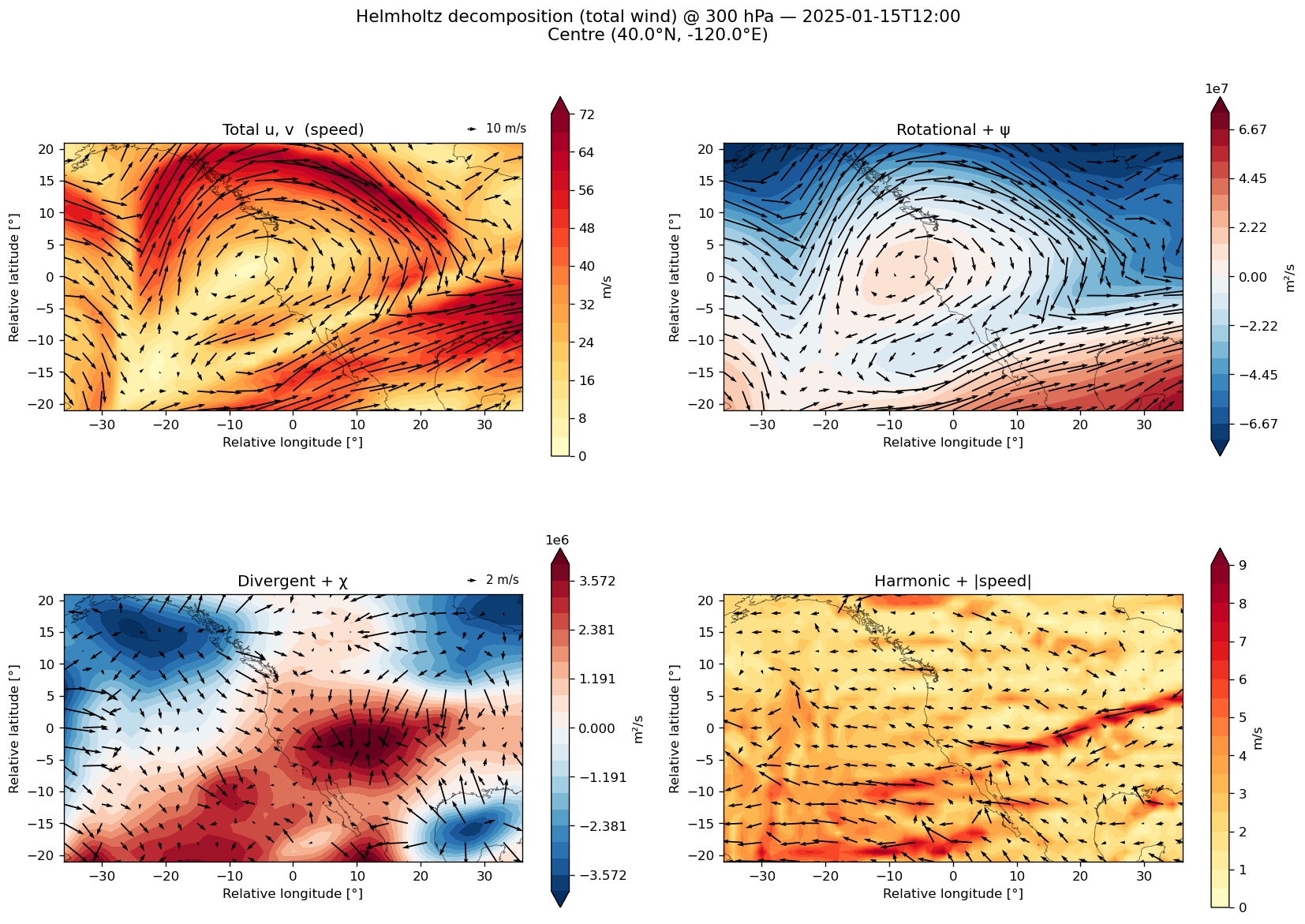
[6]:
15
6 QG omega — two-method comparison + LHR moist decomposition
Domain choices (matching production pipeline tendency.py / _sip_on_nh()):
Method |
Domain |
Reason |
|---|---|---|
SP19 |
Patch (29×49) |
Trivial scaling — |
LOG20 (SIP) |
Full NH (61×240) → extract patch |
3-D SIP solver with periodic lon BCs on full ring |
Since v2.11 the SIP meridional stencil uses the conservative cos(φ_{j±½}) flux-divergence form (Lynch 1989), replacing the tan φ coefficient form that was ill-conditioned at high latitudes; the polar Dirichlet row at φ = ±90° is set to the zonal mean of omega_b so only the geometrically well-defined m = 0 mode survives at the geometric pole. These changes substantially reduce the divergent-wind disagreement against the Helmholtz partition for high-latitude events.
Three omega components (LOG20):
Component |
Definition |
Physical meaning |
|---|---|---|
|
SIP solve with A+B terms only |
Dynamic (adiabatic) QG vertical motion |
|
|
Diabatic residual (everything not explained by adiabatic QG) |
|
|
LHR-driven vertical motion (diabatic C term) |
The LHR moist component uses θ̇_LHR ≈ (L_v/c_p)(θ/T) max(0, −ω ∂q_s/∂p) as the LHR approximation, fed into C_em = −(κ/p)∇²(J_em) where J_em = c_p θ̇_LHR T/θ.
2×3 panel: rows = methods, columns = [ω_total, ω_adia, ω_dia_res = ω_total − ω_adia]
[7]:
%%time
# ── Full-NH geostrophic wind (for LOG20 — needs periodic longitude) ──
def _geostrophic_nh(phi_3d):
    """(u_g, v_g) on the full NH grid using periodic zonal gradients."""
    ug = np.zeros_like(phi_3d)
    vg = np.zeros_like(phi_3d)
    for k in range(phi_3d.shape[0]):
        dphi_dx, dphi_dy = gradient_periodic(phi_3d[k], dx_arr, dy)
        ug[k] = -(1.0 / f_arr[:, None]) * dphi_dy
        vg[k] =  (1.0 / f_arr[:, None]) * dphi_dx
    return ug, vg

ug_snap_nh, vg_snap_nh = _geostrophic_nh(z_snap)
print(f"Full-NH geostrophic wind: max |ug|={np.abs(ug_snap_nh).max():.1f} m/s")

# ── SP19 (total, on patch — trivial adiabatic-fraction scaling) ──
t0 = time.perf_counter()
wd_sp19 = SP19_DRY_FRACTION * p_w_snap
t_sp19 = time.perf_counter() - t0

# ── LOG20 / SIP (total, on FULL NH → extract patch) — adiabatic: A+B only ──
t0 = time.perf_counter()
wd_log20_nh, info_log20 = solve_qg_omega_sip(
    ug_snap_nh, vg_snap_nh, t_snap,
    lat, lon, plevs_pa,
    center_lat=CENTER_LAT,
    omega_b=w_snap,
)
wd_log20 = patcher.extract(wd_log20_nh, i_lat, i_lon)
t_log20 = time.perf_counter() - t0

# ── Emanuel LHR approximation → w_lhr_moist (full NH) ──
# θ = T (p₀/p)^κ
kappa_val = R_DRY / 1004.0
theta_nh = t_snap * (1e5 / plevs_pa[:, None, None]) ** kappa_val

# Saturation specific humidity:  q_s = 0.622 e_s / (p - e_s)
# Bolton:  e_s [Pa] = 611.2 exp(17.67 (T-273.15) / (T - 29.65))
T_celsius = t_snap - 273.15
e_sat = 611.2 * np.exp(17.67 * T_celsius / (t_snap - 29.65))
q_sat = 0.622 * e_sat / (plevs_pa[:, None, None] - e_sat)
q_sat = np.clip(q_sat, 0, 0.1)

# ∂q_s/∂p via centred finite differences
dqs_dp = ddp(q_sat, plevs_pa)

# θ̇_LHR ≈ (L_v / c_p)(θ / T) max(0, -ω ∂q_s/∂p)
L_v = 2.501e6  # latent heat of vaporisation [J/kg]
c_p = 1004.0
condensation_rate = np.maximum(0.0, -w_snap * dqs_dp)  # >0 for ascending
theta_dot_lhr_nh = (L_v / c_p) * (theta_nh / t_snap) * condensation_rate
print(f"θ̇_LHR max = {theta_dot_lhr_nh.max():.4e} K/s, "
      f"nonzero fraction = {(theta_dot_lhr_nh > 0).mean():.1%}")

# C_em = -(κ/p) ∇²_spherical(J_em),  J_em = c_p θ̇_LHR T/θ
t0 = time.perf_counter()
C_em_nh = _compute_diabatic_rhs_emanuel(
    theta_dot_lhr_nh, t_snap, theta_nh, plevs_pa, lat, lon,
)

# Solve A+B+C_em → ω_ABC
w_abc_nh, info_abc = solve_qg_omega_sip(
    ug_snap_nh, vg_snap_nh, t_snap,
    lat, lon, plevs_pa,
    center_lat=CENTER_LAT,
    omega_b=w_snap,
    rhs_c=C_em_nh,
)
w_abc = patcher.extract(w_abc_nh, i_lat, i_lon)
t_em = time.perf_counter() - t0

# ── Three omega components ──
# w_qg_diabatic = total - adia (diabatic residual)
wm_sp19     = p_w_snap - wd_sp19
wm_log20    = p_w_snap - wd_log20     # = w_qg_diabatic for LOG20
w_qg_diabatic  = wm_log20                # alias
# w_lhr_moist = ω_ABC - ω_AB (LHR diabatic contribution, by linearity)
w_em_moist  = w_abc - wd_log20

# Extract LHR diagnostics to patch
theta_dot_lhr_patch = patcher.extract(theta_dot_lhr_nh, i_lat, i_lon)
C_em_patch = patcher.extract(C_em_nh, i_lat, i_lon)

print(f"\nSP19:  {t_sp19:.4f}s  |  LOG20 (SIP, full NH): {t_log20:.2f}s  |  Emanuel: {t_em:.2f}s")
print(f"LOG20 SIP: {info_log20['iters']} iters, "
      f"residual={info_log20['final_residual']:.2e}, "
      f"numba={info_log20['numba']}, terms={info_log20['terms']}")
print(f"ABC   SIP: {info_abc['iters']} iters, "
      f"residual={info_abc['final_residual']:.2e}, terms={info_abc['terms']}")
W_PLOT_LEV = 500
ilev_w = np.argmin(np.abs(levs_hpa - W_PLOT_LEV))
print(f"|wd_log20| max = {np.abs(wd_log20[ilev_w]).max():.4f} Pa/s")
print(f"|w_qg_diabatic| max = {np.abs(w_qg_diabatic[ilev_w]).max():.4f} Pa/s")
print(f"|w_em_moist| max = {np.abs(w_em_moist[ilev_w]).max():.4f} Pa/s")

# ── 2×3 plot: rows = [SP19, LOG20], cols = [w_total, w_adia, w_dia_res] ──
methods = [("SP19 (patch, scaling)",  p_w_snap, wd_sp19,  wm_sp19),
           ("LOG20 / SIP (full NH)",  p_w_snap, wd_log20, wm_log20)]
col_labels = ["ω_total", "ω_adia", "ω_dia_res (diabatic residual)"]

fig, axes = plt.subplots(2, 3, figsize=(18, 10))

for row, (mname, wt, wd, wm) in enumerate(methods):
    row_fields = [wt[ilev_w], wd[ilev_w], wm[ilev_w]]
    vm_row = max(np.nanpercentile(np.abs(f), 98) for f in row_fields)
    if vm_row < 1e-15:
        vm_row = 1.0
    for col, (clabel, field) in enumerate(zip(col_labels, [wt, wd, wm])):
        ax = axes[row, col]
        f2d = field[ilev_w]
        cf = ax.contourf(x_coords, y_coords, f2d,
                         levels=np.linspace(-vm_row, vm_row, 21),
                         cmap="RdBu_r", extend="both")
        overlay_coastlines(ax, **coast_kw)
        ax.set_aspect("equal")
        ax.set_title(f"{mname}: {clabel}", fontsize=11)
        plt.colorbar(cf, ax=ax, shrink=0.7, label="Pa/s")

for ax in axes.flat:
    ax.set_xlabel("Rel. lon [°]"); ax.set_ylabel("Rel. lat [°]")

fig.suptitle(f"Total omega: 2-method comparison @ {W_PLOT_LEV} hPa — {ts_str}\n"
             f"LOG20/SIP on full NH (61×240), extracted to patch",
             fontsize=14, y=0.93)
fig.tight_layout()
plt.show(); plt.close("all"); gc.collect()
Full-NH geostrophic wind: max |ug|=235.3 m/s
θ̇_LHR max = 4.2244e-03 K/s, nonzero fraction = 46.7%

SP19:  0.0000s  |  LOG20 (SIP, full NH): 1.17s  |  Emanuel: 0.37s
LOG20 SIP: 300 iters, residual=6.88e-12, numba=True, terms=AB
ABC   SIP: 300 iters, residual=4.57e-12, terms=ABC
|wd_log20| max = 0.7093 Pa/s
|w_qg_diabatic| max = 2.0354 Pa/s
|w_em_moist| max = 0.8396 Pa/s
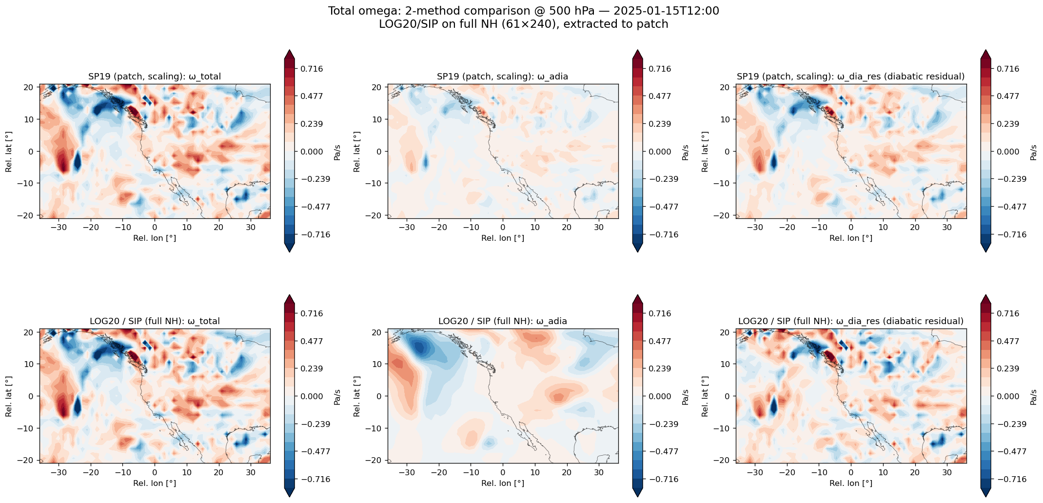
CPU times: user 2.2 s, sys: 60.4 ms, total: 2.26 s
Wall time: 2.96 s
[7]:
21
6b LHR moist decomposition: w_qg_diabatic vs w_lhr_moist
Row 1 (map at PLOT_LEV): w_total | w_qg_diabatic (= w_total - w_adia) | w_lhr_moist (= w_ABC - w_AB, own cbar range)
Row 2 (x-p cross-section at y_rel=+15°, log-p vertical axis): LHR proxy theta_dot_LHR | C_em = -(kappa/p) nabla^2 J_em (diabatic Q-term) | w_lhr_moist
The LHR approximation uses saturation-specific-humidity lapse:
[8]:
# ── 2×3 plot ──
# Row 1: w_total / w_qg_diabatic / w_lhr_moist  (map at PLOT_LEV)
#         w_lhr_moist uses its own cbar range
# Row 2: x–p cross-section at y_rel=+15  (LHR θ̇, C_em, w_lhr_moist), log-p axis

from matplotlib.ticker import ScalarFormatter

XP_YREL = 15.0  # cross-section latitude offset [°]
j_xp = np.argmin(np.abs(y_coords - XP_YREL))  # index for y_rel ≈ +15

fig, axes = plt.subplots(2, 3, figsize=(18, 11))

# ── Row 1: map view at PLOT_LEV ──
map_fields = [
    ("ω_total",     p_w_snap[ilev]),
    ("ω_qg_diabatic",  w_qg_diabatic[ilev]),
    ("ω_lhr_moist",  w_em_moist[ilev]),
]

# Shared range for w_total and w_qg_diabatic only
vm_shared = max(np.nanpercentile(np.abs(f), 98) for lbl, f in map_fields[:2])
if vm_shared < 1e-15:
    vm_shared = 1.0
# Separate range for w_em_moist
vm_em = np.nanpercentile(np.abs(w_em_moist[ilev]), 98)
if vm_em < 1e-15:
    vm_em = 1.0

for col, (label, fld) in enumerate(map_fields):
    ax = axes[0, col]
    vm_use = vm_em if col == 2 else vm_shared
    cf = ax.contourf(x_coords, y_coords, fld,
                     levels=np.linspace(-vm_use, vm_use, 21),
                     cmap="RdBu_r", extend="both")
    overlay_coastlines(ax, **coast_kw)
    ax.set_aspect("equal")
    ax.set_title(f"{label} @ {PLOT_LEV} hPa", fontsize=11)
    ax.set_xlabel("Rel. lon [°]"); ax.set_ylabel("Rel. lat [°]")
    plt.colorbar(cf, ax=ax, shrink=0.7, label="Pa/s")

# ── Row 2: x–p cross-sections at y_rel=+15, log-p axis ──
xp_fields = [
    ("θ̇_LHR [K/s]",           theta_dot_lhr_patch[:, j_xp, :], "Oranges"),
    ("C_em (Q-term) [s⁻³]",   C_em_patch[:, j_xp, :],          "RdBu_r"),
    ("ω_lhr_moist [Pa/s]",      w_em_moist[:, j_xp, :],          "RdBu_r"),
]

for col, (label, fld, cmap) in enumerate(xp_fields):
    ax = axes[1, col]
    vm_xp = np.nanpercentile(np.abs(fld), 98)
    if vm_xp < 1e-20:
        vm_xp = 1.0
    if cmap == "Oranges":
        levs_xp = np.linspace(0, vm_xp, 21)
    else:
        levs_xp = np.linspace(-vm_xp, vm_xp, 21)
    cf = ax.contourf(x_coords, levs_hpa, fld,
                     levels=levs_xp, cmap=cmap, extend="both")
    ax.set_yscale("log")
    ax.set_ylim(levs_hpa.max(), levs_hpa.min())  # high pressure at bottom
    ax.yaxis.set_major_formatter(ScalarFormatter())
    ax.yaxis.set_minor_formatter(ScalarFormatter())
    ax.set_yticks(levs_hpa)
    ax.set_title(f"{label}  (y_rel=+{XP_YREL:.0f}° section)", fontsize=10)
    ax.set_xlabel("Rel. lon [°]"); ax.set_ylabel("Pressure [hPa]")
    plt.colorbar(cf, ax=ax, shrink=0.7, label=label.split("[")[-1].rstrip("]") if "[" in label else "")

fig.suptitle(f"LHR moist decomposition @ {PLOT_LEV} hPa — {ts_str}\n"
             f"Row 1: maps  |  Row 2: x–p at y_rel=+{XP_YREL:.0f}°  |  "
             f"Centre ({CENTER_LAT}°N, {CENTER_LON}°E)",
             fontsize=13, y=0.97)
fig.tight_layout()
plt.show(); plt.close("all"); gc.collect()
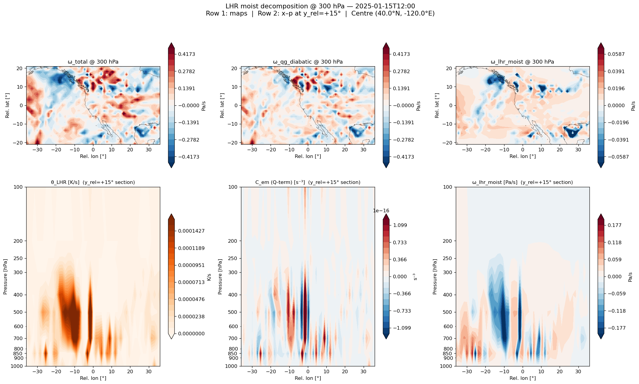
[8]:
69990
[15]:
# θ̇_LHR x–p cross-section only (converted to K/day)
from matplotlib.ticker import ScalarFormatter

XP_YREL = 15.0
j_xp = np.argmin(np.abs(y_coords - XP_YREL))

theta_lhr_kday = theta_dot_lhr_patch[:, j_xp, :] * 86400.0  # K/day
vm = np.nanpercentile(np.abs(theta_lhr_kday), 98)
if vm < 1e-12:
    vm = 1.0

fig, ax = plt.subplots(1, 1, figsize=(6, 8))
cf = ax.contourf(
    x_coords,
    levs_hpa,
    theta_lhr_kday,
    levels=np.linspace(0, vm, 21),
    cmap="Oranges",
    extend="max",
)

ax.set_yscale("log")
ax.set_ylim(levs_hpa.max(), levs_hpa.min())
ax.yaxis.set_major_formatter(ScalarFormatter())
ax.yaxis.set_minor_formatter(ScalarFormatter())
ax.set_yticks(levs_hpa)
ax.set_xlabel("Rel. lon [°]")
ax.set_ylabel("Pressure [hPa]")
ax.set_title(f"θ̇_LHR (California blocking event) — {ts_str}\n")
plt.colorbar(cf, ax=ax, shrink=0.8, label="K/day")

fig.tight_layout()
plt.show(); plt.close("all"); gc.collect()
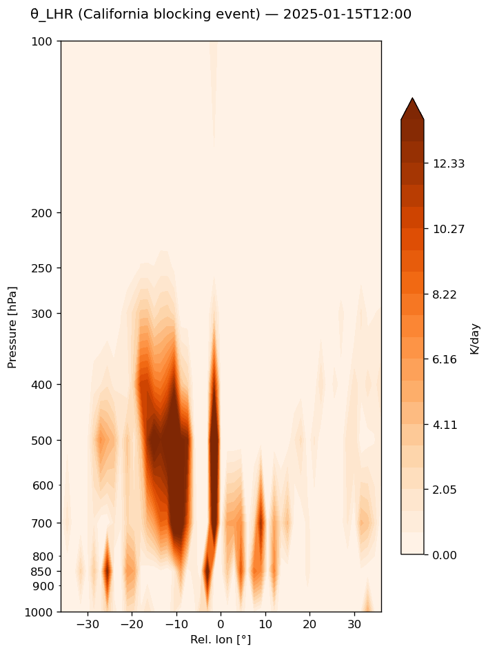
[15]:
8114
[ ]:
7 Diabatic / adiabatic divergent wind on patch
Uses decompose_omega() with ω_lhr_moist (LHR-driven) as the moist component, then recovers divergent wind for each component via independent Poisson inversions (tex Eq. 6, 15):
Both χ are solved independently using the spherical Laplacian, rather than computing one as a residual.
1×3 panel: total divergent (from Helmholtz on total wind) | adiabatic divergent | lhr-moist divergent
[10]:
%%time
# Divergent wind from w_lhr_moist and w_adia via independent Poisson
# omega_adia = wd_log20 (LOG20 A+B solve)
# omega_lhr_moist = w_em_moist (LHR contribution = omega_ABC - omega_AB)

import matplotlib.patheffects as pe

omega_dry_total = wd_log20
omega_em_moist  = w_em_moist

# Independent Poisson inversions for each component
chi_em, u_div_em, v_div_em = solve_chi_from_omega(
    omega_em_moist, patch_lat, patch_lon, plevs_pa,
)
chi_d, u_div_adiabatic, v_div_adiabatic = solve_chi_from_omega(
    omega_dry_total, patch_lat, patch_lon, plevs_pa,
)

# QG-diabatic divergent wind (from full diabatic residual omega_qg_diabatic = omega_total - omega_adia)
chi_qg, u_div_qg, v_div_qg = solve_chi_from_omega(
    w_qg_diabatic, patch_lat, patch_lon, plevs_pa,
)

# For backward compat aliases used in section 8
u_div_diabatic = u_div_em
v_div_diabatic = v_div_em
omega_diabatic_total = omega_em_moist

print(f"|u_div_lhr_moist| max = {np.abs(u_div_em[ilev]).max():.3f} m/s")
print(f"|u_div_qg_diabatic| max = {np.abs(u_div_qg[ilev]).max():.3f} m/s")
print(f"|u_div_adia|      max = {np.abs(u_div_adiabatic[ilev]).max():.3f} m/s")

# Blocking marker contour.
# Z is much cleaner than PV for this case; tmp/cali_block_z_pv_contour_diagnostic.png
# shows PV is filamentary/noisy while Z300 has a compact ridge contour over CA/East Pacific.
BLOCK_CONTOUR_VAR = "z"       # "z" or "pv"
BLOCK_CONTOUR_LEV = 300       # hPa
BLOCK_CONTOUR_VALUE = 9300.0  # m for z, PVU for pv
BLOCK_CONTOUR_LW = 3.0


def _block_contour_field(var_name, level_hpa):
    """Return the patch field, selected level index, and display label for the block contour."""
    k = int(np.argmin(np.abs(levs_hpa - level_hpa)))
    var_key = var_name.lower()
    if var_key == "z":
        field = p_z_snap[k] / G0
        unit = "m"
        label = f"Z{int(levs_hpa[k])} {BLOCK_CONTOUR_VALUE:.0f} {unit}"
    elif var_key == "pv":
        p_pv_snap = patcher.extract(pv_snap, i_lat, i_lon)
        field = p_pv_snap[k].astype(float)
        if np.nanmax(np.abs(field)) < 0.05:
            field = field / 1e-6
        unit = "PVU"
        label = f"PV{int(levs_hpa[k])} {BLOCK_CONTOUR_VALUE:.1f} {unit}"
    else:
        raise ValueError("BLOCK_CONTOUR_VAR must be 'z' or 'pv'")
    return field, k, label


block_field, block_ilev, block_label = _block_contour_field(BLOCK_CONTOUR_VAR, BLOCK_CONTOUR_LEV)
print(
    f"Block marker: {block_label}; "
    f"field range=[{np.nanmin(block_field):.2f}, {np.nanmax(block_field):.2f}]"
)


def overlay_block_contour(ax):
    """Overlay one thick white contour marking the California blocking ridge."""
    fmin = float(np.nanmin(block_field))
    fmax = float(np.nanmax(block_field))
    if not (fmin <= BLOCK_CONTOUR_VALUE <= fmax):
        print(
            f"Skipping block contour: {BLOCK_CONTOUR_VALUE:g} is outside "
            f"[{fmin:.2f}, {fmax:.2f}]"
        )
        return None
    contour = ax.contour(
        x_coords, y_coords, block_field,
        levels=[BLOCK_CONTOUR_VALUE],
        colors="white", linewidths=BLOCK_CONTOUR_LW, zorder=8,
    )
    contour_artists = getattr(contour, "collections", [contour])
    for artist in contour_artists:
        artist.set_path_effects([
            pe.Stroke(linewidth=BLOCK_CONTOUR_LW + 1.5, foreground="black", alpha=0.55),
            pe.Normal(),
        ])
    labels = ax.clabel(
        contour, levels=[BLOCK_CONTOUR_VALUE], fmt={BLOCK_CONTOUR_VALUE: block_label},
        inline=True, fontsize=8, colors="white",
    )
    for text in labels:
        text.set_path_effects([pe.Stroke(linewidth=2.0, foreground="black"), pe.Normal()])
    return contour


# 1x3 panel: divergent wind total / dry / em-moist @ PLOT_LEV
fig, axes = plt.subplots(1, 3, figsize=(18, 5))
div_panels = [
    ("Div total",       p_u_div[ilev],  p_v_div[ilev]),
    ("Div adiabatic",  u_div_adiabatic[ilev], v_div_adiabatic[ilev]),
    ("Div lhr-moist",   u_div_em[ilev],  v_div_em[ilev]),
]

for ax, (title, uk, vk) in zip(axes, div_panels):
    speed = np.sqrt(uk**2 + vk**2)
    # Scale quiver arrows proportional to max speed in each panel
    ref_speed = max(float(np.nanpercentile(speed, 98)), 0.01)
    ref_nice = float(np.round(ref_speed, -int(np.floor(np.log10(ref_speed)))))  # round to 1 sig fig
    if ref_nice < 1e-10:
        ref_nice = ref_speed
    qscale = ref_nice * 20  # 20 arrows worth across the domain

    cf = ax.contourf(x_coords, y_coords, speed, levels=20, cmap="YlOrRd", extend="max")
    q = ax.quiver(x_coords[::skip], y_coords[::skip],
                  uk[::skip, ::skip], vk[::skip, ::skip],
                  scale=qscale, width=0.003, color="k")
    overlay_block_contour(ax)
    ax.quiverkey(q, 0.88, 1.06, ref_nice, f"{ref_nice:.1f} m/s",
                 labelpos="E", fontproperties=dict(size=8))
    overlay_coastlines(ax, **coast_kw)
    ax.set_aspect("equal")
    ax.set_xlabel("Rel. lon [deg]"); ax.set_ylabel("Rel. lat [deg]")
    ax.set_title(title, fontsize=12)
    plt.colorbar(cf, ax=ax, shrink=0.7, label="m/s")

fig.suptitle(
    f"Divergent wind: total / adia / lhr-moist @ {PLOT_LEV} hPa (LOG20+LHR) - {ts_str}\n"
    f"Thick white contour: {block_label} marking CA/East Pacific block",
    fontsize=14, y=1.08,
)
fig.tight_layout()
plt.show(); plt.close("all"); gc.collect()
|u_div_lhr_moist| max = 6.420 m/s
|u_div_qg_diabatic| max = 25.642 m/s
|u_div_adia|      max = 31.891 m/s
Block marker: Z300 9300 m; field range=[8589.32, 9712.72]
CPU times: user 722 ms, sys: 7.75 ms, total: 730 ms
Wall time: 750 ms
[10]:
66929
[ ]:
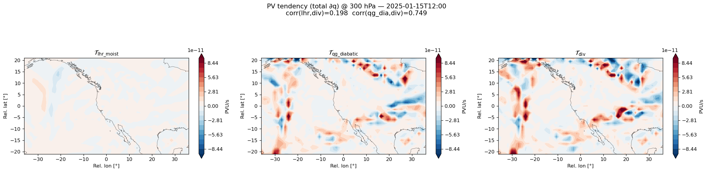
8 PV tendency on patch: three estimates
All terms use total PV gradients (\(\partial q/\partial x\), \(\partial q/\partial y\), \(\partial q/\partial p\)).
1. Indirect LHR-moist (LHR divergent wind advecting total PV):
2. QG-diabatic (full diabatic residual divergent wind from \(\omega_{\rm qg\_diabatic} = \omega - \omega_{\rm adia}\)):
3. Total divergent outflow (Helmholtz divergent wind + diabatic residual ω):
where \(\omega_{\rm dia\_res} = \omega - \omega_{\rm adia}\).
[11]:
# ── PV tendency terms on the patch ──
# Uses TOTAL PV gradient (∂q/∂x, ∂q/∂y, ∂q/∂p)
# and LHR-moist divergent wind from w_em_moist Poisson solve.

# ω_dia_res = ω_total − ω_adia  (already computed in §6 as wm_log20)
w_diabatic = wm_log20

# Indirect LHR-moist PV tendency
T_diabatic = -(u_div_diabatic * p_dpv_bar_dx
            + v_div_diabatic * p_dpv_bar_dy
            + omega_diabatic_total * p_dpv_bar_dp)

# QG-diabatic PV tendency (full diabatic divergent wind from ω_qg_diabatic Poisson)
T_qg_diabatic = -(u_div_qg * p_dpv_bar_dx
               + v_div_qg * p_dpv_bar_dy
               + w_qg_diabatic * p_dpv_bar_dp)

# Total divergent outflow PV tendency (Helmholtz div wind + ω_dia_res)
T_div = -(p_u_div * p_dpv_bar_dx
          + p_v_div * p_dpv_bar_dy
          + w_diabatic * p_dpv_bar_dp)

# ── Stats at PLOT_LEV ──
tm_lev = T_diabatic[ilev]
tq_lev = T_qg_diabatic[ilev]
td_lev = T_div[ilev]
mask = (np.abs(td_lev) > 1e-20) & np.isfinite(tm_lev) & np.isfinite(td_lev)
corr_em  = np.corrcoef(tm_lev[mask], td_lev[mask])[0, 1] if mask.sum() > 10 else np.nan
mask_qg = (np.abs(td_lev) > 1e-20) & np.isfinite(tq_lev) & np.isfinite(td_lev)
corr_qg  = np.corrcoef(tq_lev[mask_qg], td_lev[mask_qg])[0, 1] if mask_qg.sum() > 10 else np.nan
ratio_em = np.nanmean(np.abs(tm_lev)) / (np.nanmean(np.abs(td_lev)) + 1e-30)
ratio_qg = np.nanmean(np.abs(tq_lev)) / (np.nanmean(np.abs(td_lev)) + 1e-30)
print(f"At {PLOT_LEV} hPa:")
print(f"  corr(T_lhr_moist, T_div) = {corr_em:.4f}  |  |T_lhr|/|T_div| = {ratio_em:.3f}")
print(f"  corr(T_qg_diabatic, T_div) = {corr_qg:.4f}  |  |T_qd|/|T_div| = {ratio_qg:.3f}")

# ── 1×3 contourf: T_lhr_moist / T_qg_diabatic / T_div ──
fig, axes = plt.subplots(1, 3, figsize=(20, 5))

# Shared colour scale across all three
vm_pv = max(np.nanpercentile(np.abs(tm_lev), 98),
            np.nanpercentile(np.abs(tq_lev), 98),
            np.nanpercentile(np.abs(td_lev), 98))
if vm_pv < 1e-30:
    vm_pv = 1.0
levs_cf = np.linspace(-vm_pv, vm_pv, 21)

for ax, field, title in zip(axes, [tm_lev, tq_lev, td_lev],
                             [r"$\mathcal{T}_{\rm lhr\_moist}$",
                              r"$\mathcal{T}_{\rm qg\_diabatic}$",
                              r"$\mathcal{T}_{\rm div}$"]):
    cf = ax.contourf(x_coords, y_coords, field, levels=levs_cf,
                     cmap="RdBu_r", extend="both")
    overlay_coastlines(ax, **coast_kw)
    ax.set_aspect("equal")
    ax.set_xlabel("Rel. lon [°]"); ax.set_ylabel("Rel. lat [°]")
    ax.set_title(title, fontsize=13)
    plt.colorbar(cf, ax=ax, shrink=0.7, label="PVU/s")

fig.suptitle(f"PV tendency (total ∂q) @ {PLOT_LEV} hPa — {ts_str}\n"
             f"corr(lhr,div)={corr_em:.3f}  corr(qg_dia,div)={corr_qg:.3f}",
             fontsize=13, y=1.02)
fig.tight_layout()
plt.show(); plt.close("all"); gc.collect()
At 300 hPa:
  corr(T_lhr_moist, T_div) = 0.1097  |  |T_lhr|/|T_div| = 0.355
  corr(T_qg_diabatic, T_div) = 0.3675  |  |T_qd|/|T_div| = 1.749
[11]:
2323
9 Save all computed fields to NPZ
Save all patch-level fields to a compressed NPZ archive for downstream analysis. Format matches the core step2_compute_tendency_terms_blocking.py output.
[12]:
import os

out_dir = DATA_DIR
out_path = os.path.join(out_dir, "era5_step2_jan2025.npz")

# ── Vertical-average weighting (pressure thickness weights) ──
dp_weights = np.zeros(nlev)
for k in range(nlev):
    if k == 0:
        dp_weights[k] = (plevs_pa[1] - plevs_pa[0]) / 2.0
    elif k == nlev - 1:
        dp_weights[k] = (plevs_pa[-1] - plevs_pa[-2]) / 2.0
    else:
        dp_weights[k] = (plevs_pa[k+1] - plevs_pa[k-1]) / 2.0
dp_weights /= dp_weights.sum()

def wavg(f3d):
    """Pressure-weighted vertical average → 2D."""
    return np.nansum(f3d * dp_weights[:, None, None], axis=0)

np.savez_compressed(
    out_path,
    # ── Metadata ──
    Y_rel=Y_rel,
    X_rel=X_rel,
    levels=levs_hpa,
    plevs_pa=plevs_pa,
    center_lat=CENTER_LAT,
    center_lon=CENTER_LON,
    timestamp=ts_str,
    qg_method="log20",
    # ── Patch meteorological fields (3D: nlev, nlat_p, nlon_p) ──
    t_snap=p_t_snap,
    z_snap=p_z_snap,
    w_snap=p_w_snap,
    u_snap=p_u_snap,
    v_snap=p_v_snap,
    # ── Helmholtz wind (3D, spherical FFT Laplacian) ──
    u_rot=p_u_rot,
    v_rot=p_v_rot,
    u_div=p_u_div,
    v_div=p_v_div,
    u_har=p_u_har,
    v_har=p_v_har,
    psi=p_psi,
    chi=p_chi,
    # ── Geostrophic wind (3D) ──
    ug_snap=p_ug_snap,
    vg_snap=p_vg_snap,
    # ── PV derivatives (3D) ──
    dpv_bar_dx=p_dpv_bar_dx,
    dpv_bar_dy=p_dpv_bar_dy,
    dpv_bar_dp=p_dpv_bar_dp,
    # ── QG omega: adiabatic (A+B), full (A+B+C_em) ──
    omega_dry_sp19=wd_sp19,
    omega_dry_log20=wd_log20,
    omega_moist_sp19=wm_sp19,
    omega_moist_log20=wm_log20,
    # ── Three components: w_adia, w_qg_diabatic, w_lhr_moist ──
    omega_dry_total=wd_log20,
    w_qg_diabatic=w_qg_diabatic,
    w_em_moist=w_em_moist,
    # ── LHR diagnostics (patch) ──
    theta_dot_lhr=theta_dot_lhr_patch,
    C_em=C_em_patch,
    # ── LHR/adiabatic divergent wind from w_lhr_moist Poisson (3D) ──
    u_div_diabatic=u_div_diabatic,
    v_div_diabatic=v_div_diabatic,
    u_div_adiabatic=u_div_adiabatic,
    v_div_adiabatic=v_div_adiabatic,
    omega_diabatic_total=omega_diabatic_total,
    # ── PV tendency (3D) ──
    T_diabatic=T_diabatic,
    T_div=T_div,
    # ── Vertical averages (2D) ──
    T_diabatic_wavg=wavg(T_diabatic),
    T_div_wavg=wavg(T_div),
    u_rot_wavg=wavg(p_u_rot),
    v_rot_wavg=wavg(p_v_rot),
    u_div_wavg=wavg(p_u_div),
    v_div_wavg=wavg(p_v_div),
    u_div_diabatic_wavg=wavg(u_div_diabatic),
    v_div_diabatic_wavg=wavg(v_div_diabatic),
)

print(f"Saved → {out_path}  ({os.path.getsize(out_path)/1e6:.1f} MB)")
Saved → era5_jan2025/era5_step2_jan2025.npz (1.9 MB)