01 — Rossby Wave Breaking & Derivative Operators (Live ERA5)
This notebook downloads real ERA5 data from the CDS API and demonstrates the full pvtend workflow from scratch:
Download ERA5 Jan 5-25 2025 (6 vars, 9 levels, 1.5° NH hourly) via CDS
Load hourly climatology and compute anomalies
Grid setup (
NHGrid) and event-centred patch extraction (EventPatch)PV derivative computation (
ddx,ddy,ddp)Circumpolar-first RWB detection: find circumpolar Z contours on the full NH field, crop to event patch, detect overturning, classify AWB/CWB via path-order (no tilt fallback)
[1]:
import warnings
from pathlib import Path

import numpy as np
import xarray as xr
import matplotlib.pyplot as plt
import cdsapi
import cartopy.io.shapereader as shpreader
from shapely.geometry import box as shapely_box

from pvtend import NHGrid, EventPatch, ddx, ddy, ddp, R_EARTH, H_SCALE
from pvtend.rwb import (detect_rwb_events, RWBConfig, reduce_to_2d,
                        circumpolar_contours, crop_contour_to_patch,
                        sampled_longest_contours)
from pvtend.io import load_era5_month
from pvtend.constants import DEFAULT_LEVELS, CLIM_VARIABLES

warnings.filterwarnings("ignore", category=xr.SerializationWarning)


def overlay_coastlines(ax, centre_lat, centre_lon, xlim, ylim,
                       lw=0.5, color="k", alpha=0.6, resolution="50m"):
    """Overlay coastlines in event-relative coordinates."""
    shp = shpreader.natural_earth(resolution, "physical", "coastline")
    reader = shpreader.Reader(shp)
    clip = shapely_box(centre_lon + xlim[0], centre_lat + ylim[0],
                       centre_lon + xlim[1], centre_lat + ylim[1])
    for geom in reader.geometries():
        clipped = geom.intersection(clip)
        if clipped.is_empty:
            continue
        parts = clipped.geoms if hasattr(clipped, "geoms") else [clipped]
        for part in parts:
            if hasattr(part, "coords"):
                coords = np.array(part.coords)
                ax.plot(coords[:, 0] - centre_lon,
                        coords[:, 1] - centre_lat,
                        color=color, lw=lw, alpha=alpha)
1 Download ERA5 Jan 2025 from CDS
Download 6 variables × 9 pressure levels, 1.5° resolution, Northern Hemisphere (0–90 °N), hourly, for 5–25 January 2025. Each variable is saved as a separate NetCDF file in examples/era5_jan2025/.
[2]:
# ── Configuration ──
DATA_DIR = Path("/net/flood/data2/users/x_yan/pvtend/examples/era5_jan2025")
CLIM_DIR = Path("/net/flood/data2/users/x_yan/era/clim")
DATA_DIR.mkdir(parents=True, exist_ok=True)

YEAR, MONTH = 2025, 1
DAYS = [f"{d:02d}" for d in range(5, 26)]          # Jan 5-25
HOURS = [f"{h:02d}:00" for h in range(24)]
LEVELS = [str(l) for l in DEFAULT_LEVELS]           # 1000..100
GRID = "1.5/1.5"
AREA = [90, -180, 0, 180]                           # NH

CDS_VARS = {
    "u": "u_component_of_wind",
    "v": "v_component_of_wind",
    "w": "vertical_velocity",
    "t": "temperature",
    "pv": "potential_vorticity",
    "z": "geopotential",
    "q": "specific_humidity",
}

# ── Download (skip if files already exist) ──
c = cdsapi.Client()
for short, long_name in CDS_VARS.items():
    out_path = DATA_DIR / f"era5_{short}_{YEAR}_{MONTH:02d}.nc"
    if out_path.exists():
        print(f"{out_path.name} already exists, skipping")
        continue
    print(f"downloading {short} ({long_name}) …")
    c.retrieve(
        "reanalysis-era5-pressure-levels",
        {
            "product_type": "reanalysis",
            "variable": long_name,
            "year": str(YEAR),
            "month": f"{MONTH:02d}",
            "day": DAYS,
            "time": HOURS,
            "pressure_level": LEVELS,
            "grid": GRID,
            "area": AREA,
            "format": "netcdf",
        },
        str(out_path),
    )
    print(f"{out_path.name}  ({out_path.stat().st_size / 1e6:.0f} MB)")

print(f"\nAll files in {DATA_DIR}:")
for f in sorted(DATA_DIR.glob("*.nc")):
    print(f"  {f.name}  ({f.stat().st_size / 1e6:.0f} MB)")
era5_u_2025_01.nc already exists, skipping
era5_v_2025_01.nc already exists, skipping
era5_w_2025_01.nc already exists, skipping
era5_t_2025_01.nc already exists, skipping
era5_pv_2025_01.nc already exists, skipping
era5_z_2025_01.nc already exists, skipping
era5_q_2025_01.nc already exists, skipping

All files in /net/flood/data2/users/x_yan/pvtend/examples/era5_jan2025:
  era5_pv_2025_01.nc  (151 MB)
  era5_q_2025_01.nc  (266 MB)
  era5_t_2025_01.nc  (121 MB)
  era5_u_2025_01.nc  (163 MB)
  era5_v_2025_01.nc  (169 MB)
  era5_w_2025_01.nc  (173 MB)
  era5_z_2025_01.nc  (118 MB)
2 Load ERA5 snapshot & climatology → anomalies
Select a single timestamp (Jan 15 12Z) and subtract the hourly climatology to obtain anomaly fields for all 6 variables.
[3]:
# ── Target timestamp ──
TARGET_DAY, TARGET_HOUR = 15, 12
TARGET_TS = np.datetime64(f"{YEAR}-{MONTH:02d}-{TARGET_DAY:02d}T{TARGET_HOUR:02d}:00")

# ── Load downloaded ERA5 data for target time ──
ds = load_era5_month(DATA_DIR, YEAR, MONTH, list(CDS_VARS.keys()))
snap = ds.sel(valid_time=TARGET_TS, method="nearest")
print(f"Snapshot time : {snap.valid_time.values}")
print(f"Levels (hPa)  : {snap.pressure_level.values}")
print(f"Grid          : {snap.latitude.size} lat × {snap.longitude.size} lon")

# ── Load January climatology for this day & hour ──
clim_parts = []
for var in CLIM_VARIABLES:
    fp = CLIM_DIR / f"era5_hourly_clim_1990-2020_jan_{var}.nc"
    if not fp.exists():
        print(f"clim missing: {fp.name}")
        continue
    cv = xr.open_dataset(fp)
    clim_parts.append(cv.sel(day=TARGET_DAY, hour=TARGET_HOUR, month=1))
clim = xr.merge(clim_parts)

# ── Compute anomalies ──
anom = {}
for var in CLIM_VARIABLES:
    if var in snap and var in clim:
        anom[var] = snap[var].values - clim[var].values  # (nlev, nlat, nlon)
        print(f"  {var} anom range: [{anom[var].min():.3g}, {anom[var].max():.3g}]")

lat = snap.latitude.values
lon = snap.longitude.values
levels = snap.pressure_level.values
print(f"\nAnomaly fields computed for {len(anom)} variables")
Snapshot time : 2025-01-15T12:00:00.000000000
Levels (hPa)  : [1000.  850.  700.  500.  400.  300.  250.  200.  100.]
Grid          : 61 lat × 240 lon
clim missing: era5_hourly_clim_1990-2020_jan_q.nc
/tmp/ipykernel_2498492/505610482.py:21: FutureWarning: In a future version of xarray the default value for compat will change from compat='no_conflicts' to compat='override'. This is likely to lead to different results when combining overlapping variables with the same name. To opt in to new defaults and get rid of these warnings now use `set_options(use_new_combine_kwarg_defaults=True) or set compat explicitly.
  clim = xr.merge(clim_parts)
  u anom range: [-55, 58.9]
  v anom range: [-52.6, 53.1]
  w anom range: [-6.24, 3.14]
  t anom range: [-17.6, 24]
  pv anom range: [-3.77e-05, 5.75e-05]
  z anom range: [-4.29e+03, 5.37e+03]

Anomaly fields computed for 6 variables
3 Grid helper & event-centred patch extraction
Centre the ±21° lat × ±36° lon patch on California / East Pacific (37°N, 230°E = −120°), then extract all variable fields.
[4]:
# ── NH grid (1.5° resolution, lat descending 90→0) ──
grid = NHGrid(lat=lat, lon=lon)
patcher = EventPatch(grid)          # default: ±21° lat, ±36° lon

# ── Fixed centre: California / East Pacific ──
centre_lat, centre_lon = 40.0, -120.0
print(f"Patch centre: {centre_lat:.1f}°N, {centre_lon:.1f}°E")

# ── Extract patches for all variables ──
ilat, ilon, ok = patcher.nearest_idx(centre_lat, centre_lon)
assert ok, f"Patch does not fit at ({centre_lat}, {centre_lon})"

patches = {}
for var in CLIM_VARIABLES:
    if var in anom:
        patches[var] = patcher.extract(anom[var], ilat, ilon)      # (nlev, nlat_p, nlon_p)
    if var in snap:
        patches[f"{var}_raw"] = patcher.extract(snap[var].values, ilat, ilon)

Y_rel, X_rel = patcher.relative_grid()
x_coords = X_rel[0, :]    # 1D relative longitude
y_coords = Y_rel[:, 0]    # 1D relative latitude

# Grid spacings on the patch (ascending lat)
patch_lat = lat[ilat] + y_coords  # approximate absolute lats for dx
dx_patch = np.deg2rad(grid.dlon) * R_EARTH * np.cos(np.deg2rad(patch_lat))
dx_patch = np.maximum(dx_patch, grid.dy * 0.01)
dy_patch = grid.dy

print(f"Patch shape   : {patches['pv'].shape}")
print(f"Absolute box  : lat [{centre_lat-21:.0f}°, {centre_lat+21:.0f}°N], "
      f"lon [{centre_lon-36:.0f}°, {centre_lon+36:.0f}°E]")
print(f"Relative box  : x=[{x_coords.min():.0f}°, {x_coords.max():.0f}°], "
      f"y=[{y_coords.min():.0f}°, {y_coords.max():.0f}°]")
Patch centre: 40.0°N, -120.0°E
Patch shape   : (9, 29, 49)
Absolute box  : lat [19°, 61°N], lon [-156°, -84°E]
Relative box  : x=[-36°, 36°], y=[-21°, 21°]
4 Compute PV derivatives on the patch
[ ]:
pv_total = patches["pv_raw"]  # (9, nlat_p, nlon_p) — TOTAL PV on patch

# ∂PV/∂x and ∂PV/∂y on total PV (iterate over levels)
pv_dx = np.stack([ddx(pv_total[k], dx_patch, periodic=False) for k in range(len(levels))])
pv_dy = np.stack([ddy(pv_total[k], dy_patch) for k in range(len(levels))])

# ∂²PV/∂x∂y — quadrupole base (cross derivative of total PV)
pv_dxdy = np.stack([ddx(pv_dy[k], dx_patch, periodic=False) for k in range(len(levels))])

# ∂²PV/∂x² and ∂²PV/∂y² — needed for strain and Laplacian bases
pv_dxdx = np.stack([ddx(pv_dx[k], dx_patch, periodic=False) for k in range(len(levels))])
pv_dydy = np.stack([ddy(pv_dy[k], dy_patch) for k in range(len(levels))])

print(f"∂PV/∂x    shape: {pv_dx.shape},  range: [{pv_dx.min():.3g}, {pv_dx.max():.3g}]")
print(f"∂PV/∂y    shape: {pv_dy.shape},  range: [{pv_dy.min():.3g}, {pv_dy.max():.3g}]")
print(f"∂²PV/∂x∂y shape: {pv_dxdy.shape},  range: [{pv_dxdy.min():.3g}, {pv_dxdy.max():.3g}]")
print(f"∂²PV/∂x²  shape: {pv_dxdx.shape},  range: [{pv_dxdx.min():.3g}, {pv_dxdx.max():.3g}]")
print(f"∂²PV/∂y²  shape: {pv_dydy.shape},  range: [{pv_dydy.min():.3g}, {pv_dydy.max():.3g}]")
∂PV/∂x    shape: (9, 29, 49),  range: [-3.61e-10, 3.73e-10]
∂PV/∂y    shape: (9, 29, 49),  range: [-1.19e-10, 3.6e-10]
∂²PV/∂x∂y shape: (9, 29, 49),  range: [-2.24e-15, 2.29e-15]
[6]:
# Pressure derivative  ∂PV/∂p (total field)
plevs_pa = levels.astype(float) * 100.0  # hPa → Pa
pv_dp = ddp(pv_total, plevs_pa)

print(f"∂PV/∂p shape: {pv_dp.shape}")
print(f"∂PV/∂p range: [{pv_dp.min():.3g}, {pv_dp.max():.3g}]")
∂PV/∂p shape: (9, 29, 49)
∂PV/∂p range: [-1.38e-09, 2.23e-09]
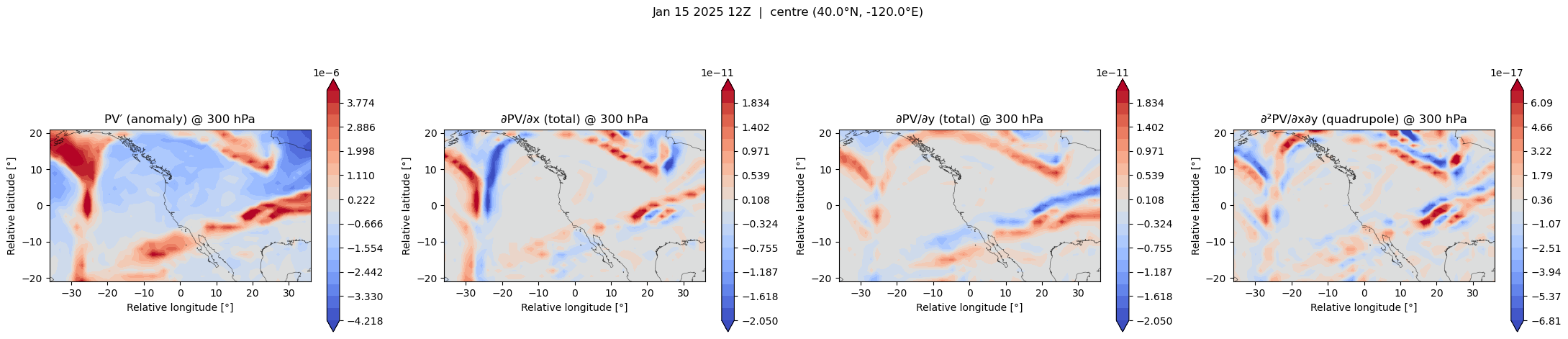
5 Visualise PV anomaly, total-field gradients & 2nd-order bases at 300 hPa
[ ]:
ilev = int(np.abs(levels - 300).argmin())
pv_anom_patch = patches["pv"]  # anomaly for first panel

fig, axes = plt.subplots(3, 3, figsize=(22, 15))
kw = dict(cmap="coolwarm", origin="lower", extend="both")
coast_kw = dict(centre_lat=centre_lat, centre_lon=centre_lon,
                xlim=(x_coords.min(), x_coords.max()),
                ylim=(y_coords.min(), y_coords.max()))

# --- Row 1: PV anomaly + 1st-order gradients ---
# Panel 1: PV anomaly
vmax_a = np.nanpercentile(np.abs(pv_anom_patch[ilev]), 98)
im0 = axes[0, 0].contourf(x_coords, y_coords, pv_anom_patch[ilev],
                           levels=np.linspace(-vmax_a, vmax_a, 20), **kw)
axes[0, 0].set_title("PV′ (anomaly) @ 300 hPa")
plt.colorbar(im0, ax=axes[0, 0], shrink=0.8)

# Panel 2: dPV/dx (total field)
vmax_g = np.nanpercentile(np.abs(pv_dx[ilev]), 98)
im1 = axes[0, 1].contourf(x_coords, y_coords, pv_dx[ilev],
                           levels=np.linspace(-vmax_g, vmax_g, 20), **kw)
axes[0, 1].set_title("∂PV/∂x (total) @ 300 hPa")
plt.colorbar(im1, ax=axes[0, 1], shrink=0.8)

# Panel 3: dPV/dy (total field)
im2 = axes[0, 2].contourf(x_coords, y_coords, pv_dy[ilev],
                           levels=np.linspace(-vmax_g, vmax_g, 20), **kw)
axes[0, 2].set_title("∂PV/∂y (total) @ 300 hPa")
plt.colorbar(im2, ax=axes[0, 2], shrink=0.8)

# --- Row 2: 2nd-order derivative bases ---
# Panel 4: d2PV/dxdy (quadrupole / shear deformation)
vmax_q = np.nanpercentile(np.abs(pv_dxdy[ilev]), 98)
im3 = axes[1, 0].contourf(x_coords, y_coords, pv_dxdy[ilev],
                           levels=np.linspace(-vmax_q, vmax_q, 20), **kw)
axes[1, 0].set_title("∂²PV/∂x∂y (shear Φ₄) @ 300 hPa")
plt.colorbar(im3, ax=axes[1, 0], shrink=0.8)

# Panel 5: d2PV/dx2 - d2PV/dy2 (normal strain)
strain = pv_dxdx[ilev] - pv_dydy[ilev]
vmax_s = np.nanpercentile(np.abs(strain), 98)
im4 = axes[1, 1].contourf(x_coords, y_coords, strain,
                           levels=np.linspace(-vmax_s, vmax_s, 20), **kw)
axes[1, 1].set_title("∂²PV/∂x² − ∂²PV/∂y² (strain Φ₅) @ 300 hPa")
plt.colorbar(im4, ax=axes[1, 1], shrink=0.8)

# Panel 6: d2PV/dx2 + d2PV/dy2 (Laplacian)
laplacian = pv_dxdx[ilev] + pv_dydy[ilev]
vmax_l = np.nanpercentile(np.abs(laplacian), 98)
im5 = axes[1, 2].contourf(x_coords, y_coords, laplacian,
                           levels=np.linspace(-vmax_l, vmax_l, 20), **kw)
axes[1, 2].set_title("∇²PV (Laplacian Φ₆) @ 300 hPa")
plt.colorbar(im5, ax=axes[1, 2], shrink=0.8)

# --- Row 3: Individual 2nd-order derivatives ---
# Panel 7: d2PV/dx2
vmax_xx = np.nanpercentile(np.abs(pv_dxdx[ilev]), 98)
im6 = axes[2, 0].contourf(x_coords, y_coords, pv_dxdx[ilev],
                           levels=np.linspace(-vmax_xx, vmax_xx, 20), **kw)
axes[2, 0].set_title("∂²PV/∂x² @ 300 hPa")
plt.colorbar(im6, ax=axes[2, 0], shrink=0.8)

# Panel 8: d2PV/dy2
vmax_yy = np.nanpercentile(np.abs(pv_dydy[ilev]), 98)
im7 = axes[2, 1].contourf(x_coords, y_coords, pv_dydy[ilev],
                           levels=np.linspace(-vmax_yy, vmax_yy, 20), **kw)
axes[2, 1].set_title("∂²PV/∂y² @ 300 hPa")
plt.colorbar(im7, ax=axes[2, 1], shrink=0.8)

# Panel 9: d2PV/dxdy (duplicate of Φ₄ for completeness)
im8 = axes[2, 2].contourf(x_coords, y_coords, pv_dxdy[ilev],
                           levels=np.linspace(-vmax_q, vmax_q, 20), **kw)
axes[2, 2].set_title("∂²PV/∂x∂y @ 300 hPa")
plt.colorbar(im8, ax=axes[2, 2], shrink=0.8)

for ax in axes.ravel():
    overlay_coastlines(ax, **coast_kw)
    ax.set_xlabel("Relative longitude [°]")
    ax.set_ylabel("Relative latitude [°]")
    ax.set_aspect("equal")
fig.suptitle(f"Jan 15 2025 12Z  |  centre ({centre_lat:.1f}°N, {centre_lon:.1f}°E)\n"
             "Row 1: PV anomaly + 1st-order gradients  |  Row 2: Combined bases  |  Row 3: Individual 2nd-order", y=1.02)
fig.tight_layout()
plt.show()
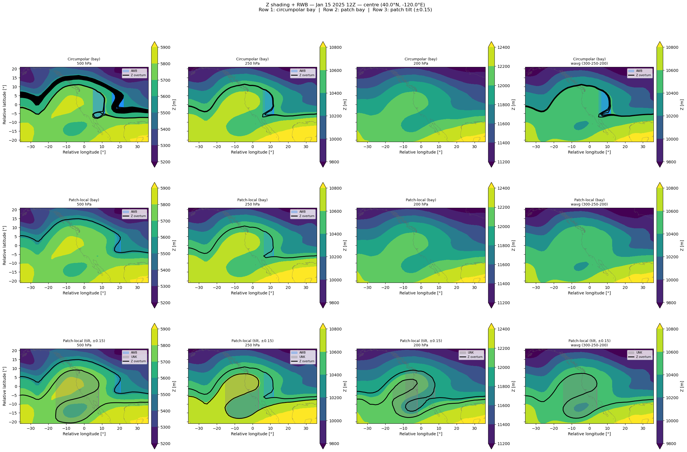
6 Circumpolar-first RWB detection at 500 / 250 / 200 hPa and weighted-average
Two-method API — default method="bay" (path-order, no tilt fallback):
For each pressure level, extract the full-NH Z field.
Find all circumpolar Z contours spanning the entire longitude range.
Crop each circumpolar contour to the event-centred patch.
Detect overturning (folding) within the patch via meridian crossing counts.
Classify AWB/CWB via path-order — ambiguous bays remain “UNK”.
Shading: Z (geopotential height in metres) with Z-contour RWB overlays.
[8]:
# ── Prepare PV and Z fields on the patch ──
pv_total = patches["pv_raw"]  # (9, nlat_p, nlon_p)

level_modes = [500, 250, 200, "wavg"]
pv_2d = {}
z_2d  = {}   # Z (geopotential height, m) on patch — for shading

# Geopotential height in metres for wavg weighting (z / g)
z_patch = patches.get("z_raw")   # raw z (geopotential), (nlev, nlat_p, nlon_p)
z_m = z_patch / 9.81 if z_patch is not None else None

# Subset to 300/250/200 hPa for the wavg
wavg_idx = np.array([int(np.abs(levels - l).argmin()) for l in [300, 250, 200]])
pv_wavg_sub = pv_total[wavg_idx]          # (3, nlat_p, nlon_p)
z_wavg_sub = z_m[wavg_idx] if z_m is not None else None

for mode in level_modes:
    if mode == "wavg":
        pv_2d[mode] = reduce_to_2d(pv_wavg_sub, np.array([300, 250, 200]),
                                    "wavg", z3d_m=z_wavg_sub, H_SCALE=H_SCALE)
        z_2d[mode]  = reduce_to_2d(z_wavg_sub, np.array([300, 250, 200]),
                                    "wavg", z3d_m=z_wavg_sub, H_SCALE=H_SCALE)
    else:
        pv_2d[mode] = reduce_to_2d(pv_total, levels, mode)
        z_2d[mode]  = reduce_to_2d(z_m, levels, mode)

# ── Full-NH Z fields for circumpolar contour extraction ──
z_full_nh = snap["z"].values / 9.81   # (nlev, nlat, nlon) in metres
lat_nh = lat                           # full NH lat array
lon_nh = lon                           # full NH lon array

cfg = RWBConfig(try_levels=300, min_vertices=20, area_min_deg2=20.0)

# ── Run RWB detection: (A) circumpolar, (B) patch-local, (C) tilt ──
rwb_circ  = {}   # circumpolar-first, bay method
rwb_patch = {}   # patch-local, bay method
rwb_tilt  = {}   # patch-local, tilt method (±0.15 dead zone)

for mode in level_modes:
    if mode == "wavg":
        z_nh_2d = reduce_to_2d(z_full_nh[wavg_idx], np.array([300, 250, 200]),
                                "wavg", z3d_m=z_full_nh[wavg_idx], H_SCALE=H_SCALE)
    else:
        z_nh_2d = reduce_to_2d(z_full_nh, levels, mode)

    # (A) Circumpolar-first, bay
    ev_circ = detect_rwb_events(
        z_2d[mode], x_coords, y_coords, cfg=cfg,
        field_nh=z_nh_2d,
        lat_nh=lat_nh, lon_nh=lon_nh,
        centre_lat=centre_lat, centre_lon=centre_lon,
        method="bay",
    )
    rwb_circ[mode] = ev_circ

    # (B) Patch-local, bay
    ev_patch = detect_rwb_events(
        z_2d[mode], x_coords, y_coords, cfg=cfg,
        method="bay",
    )
    rwb_patch[mode] = ev_patch

    # (C) Patch-local, tilt (±0.15 dead zone)
    ev_tilt = detect_rwb_events(
        z_2d[mode], x_coords, y_coords, cfg=cfg,
        method="tilt",
    )
    rwb_tilt[mode] = ev_tilt

    label = "wavg" if mode == "wavg" else f"{mode} hPa"
    nc = lambda evs, t: sum(1 for e in evs if e["wb_type"] == t)
    print(f"  {label:>8s}:  circ {len(ev_circ)} (AWB={nc(ev_circ,'AWB')}, "
          f"CWB={nc(ev_circ,'CWB')}, UNK={nc(ev_circ,'UNK')})  |  "
          f"patch {len(ev_patch)} (AWB={nc(ev_patch,'AWB')}, "
          f"CWB={nc(ev_patch,'CWB')}, UNK={nc(ev_patch,'UNK')})  |  "
          f"tilt {len(ev_tilt)} (AWB={nc(ev_tilt,'AWB')}, "
          f"CWB={nc(ev_tilt,'CWB')}, UNK={nc(ev_tilt,'UNK')})")

# Show circumpolar contour counts
for mode in level_modes:
    if mode == "wavg":
        z_nh_2d = reduce_to_2d(z_full_nh[wavg_idx], np.array([300, 250, 200]),
                                "wavg", z3d_m=z_full_nh[wavg_idx], H_SCALE=H_SCALE)
    else:
        z_nh_2d = reduce_to_2d(z_full_nh, levels, mode)
    circ = circumpolar_contours(z_nh_2d, lat_nh, lon_nh,
                                try_levels=cfg.try_levels,
                                min_vertices=cfg.min_vertices)
    label = "wavg" if mode == "wavg" else f"{mode} hPa"
    print(f"  {label:>8s}: {len(circ)} circumpolar contours found on full NH")
   500 hPa:  circ 22 (AWB=22, CWB=0, UNK=0)  |  patch 1 (AWB=1, CWB=0, UNK=0)  |  tilt 2 (AWB=1, CWB=0, UNK=1)
   250 hPa:  circ 2 (AWB=2, CWB=0, UNK=0)  |  patch 1 (AWB=1, CWB=0, UNK=0)  |  tilt 2 (AWB=1, CWB=0, UNK=1)
   200 hPa:  circ 0 (AWB=0, CWB=0, UNK=0)  |  patch 0 (AWB=0, CWB=0, UNK=0)  |  tilt 2 (AWB=0, CWB=0, UNK=2)
      wavg:  circ 3 (AWB=3, CWB=0, UNK=0)  |  patch 0 (AWB=0, CWB=0, UNK=0)  |  tilt 1 (AWB=0, CWB=0, UNK=1)
   500 hPa: 211 circumpolar contours found on full NH
   250 hPa: 250 circumpolar contours found on full NH
   200 hPa: 263 circumpolar contours found on full NH
      wavg: 249 circumpolar contours found on full NH
[9]:
from matplotlib.lines import Line2D

fig, axes = plt.subplots(3, 4, figsize=(24, 16), sharey=True)
colors = {"AWB": "dodgerblue", "CWB": "tomato", "UNK": "gray"}
coast_kw = dict(centre_lat=centre_lat, centre_lon=centre_lon,
                xlim=(x_coords.min(), x_coords.max()),
                ylim=(y_coords.min(), y_coords.max()))

row_labels = ["Circumpolar (bay)", "Patch-local (bay)", "Patch-local (tilt, ±0.15)"]
rwb_dicts  = [rwb_circ, rwb_patch, rwb_tilt]

for row, (rwb_results, row_lbl) in enumerate(zip(rwb_dicts, row_labels)):
    for col, mode in enumerate(level_modes):
        ax = axes[row, col]

        # ── Shade Z (geopotential height in metres) ──
        z_field = z_2d[mode]
        cf = ax.contourf(x_coords, y_coords, z_field,
                         cmap="viridis", extend="both")

        # ── Overlay contours ──
        if row == 0:
            # Circumpolar: get NH contours, crop to patch
            if mode == "wavg":
                z_nh_2d = reduce_to_2d(z_full_nh[wavg_idx], np.array([300, 250, 200]),
                                        "wavg", z3d_m=z_full_nh[wavg_idx], H_SCALE=H_SCALE)
            else:
                z_nh_2d = reduce_to_2d(z_full_nh, levels, mode)
            circ = circumpolar_contours(z_nh_2d, lat_nh, lon_nh,
                                        try_levels=cfg.try_levels,
                                        min_vertices=cfg.min_vertices)
            half_dlat = float(np.max(np.abs(y_coords)))
            half_dlon = float(np.max(np.abs(x_coords)))
            contours = []
            for cc in circ:
                cropped = crop_contour_to_patch(cc, centre_lat, centre_lon,
                                                half_dlat=half_dlat, half_dlon=half_dlon)
                if cropped is not None:
                    contours.append(cropped)
        else:
            # Patch-local: sampled_longest_contours on patch Z
            contours = sampled_longest_contours(z_field, x_coords, y_coords,
                                                 try_levels=cfg.try_levels,
                                                 max_keep=12,
                                                 min_vertices=cfg.min_vertices)

        contour_by_lev = {c["lev"]: c for c in contours}

        # Overlay overturning Z contours (BLACK) + RWB polygons
        plotted_levels = set()
        for ev in rwb_results[mode]:
            clev = ev["contour_level"]
            if clev not in plotted_levels and clev in contour_by_lev:
                cline = contour_by_lev[clev]
                ax.plot(cline["x"], cline["y"],
                        color="k", lw=2.0, zorder=3)
                plotted_levels.add(clev)

            c = colors.get(ev["wb_type"], "gray")
            ax.fill(ev["polygon_x"], ev["polygon_y"], alpha=0.3, color=c,
                    label=ev["wb_type"])
            ax.plot(ev["polygon_x"], ev["polygon_y"], color=c, lw=1.5)

        overlay_coastlines(ax, **coast_kw, color="0.4")
        plt.colorbar(cf, ax=ax, shrink=0.8, pad=0.02, label="Z [m]")

        lev_label = "wavg (300-250-200)" if mode == "wavg" else f"{mode} hPa"
        ax.set_title(f"{row_lbl}\n{lev_label}", fontsize=9)
        ax.set_xlabel("Relative longitude [°]")
        ax.set_aspect("equal")

        handles, labels_ = ax.get_legend_handles_labels()
        by_label = dict(zip(labels_, handles))
        if plotted_levels:
            by_label["Z overturn"] = Line2D([0], [0], color="k", lw=2)
        if by_label:
            ax.legend(by_label.values(), by_label.keys(),
                      loc="upper right", fontsize=7)

    axes[row, 0].set_ylabel("Relative latitude [°]")

fig.suptitle(f"Z shading + RWB — Jan 15 2025 12Z — "
             f"centre ({centre_lat:.1f}°N, {centre_lon:.1f}°E)\n"
             f"Row 1: circumpolar bay  |  Row 2: patch bay  |  "
             f"Row 3: patch tilt (±0.15)", y=1.01)
fig.tight_layout()
plt.show()